Time Series Jiří Holčík
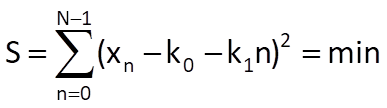
The following holds for a quadratic trend estimate:
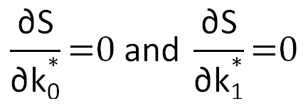
and the defining system of equations to determine the optimal values of coefficients is
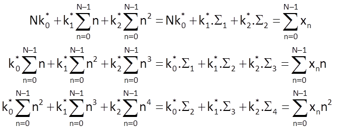
As a consequence, we can write the following for coefficients of this model:
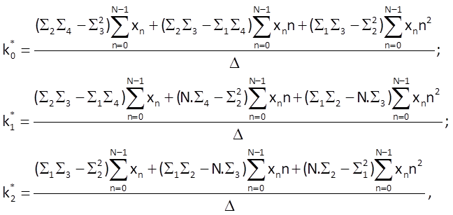
where Δ = N.(Σ2Σ4 – Σ32) + Σ1(Σ2Σ3 – Σ1Σ4) +Σ2(Σ1Σ3 – Σ22) .
Finally, we can determine the predicted value of the Mth sample xpM by
Note
When solving problems in practice, it is usually not convenient to use higher-order polynomials, especially if it is necessary to use the developed model for the prediction of time series values. With regard to the computation of optimum values of coefficients, the computational complexity grows tremendously for higher-order polynomials, as shown by the comparison of computational complexity in the three above-mentioned cases. Moreover, although the approximation by higher-order polynomials is more accurate within a known interval, it is significantly less reliable beyond this interval, as shown in Figure 9.3.
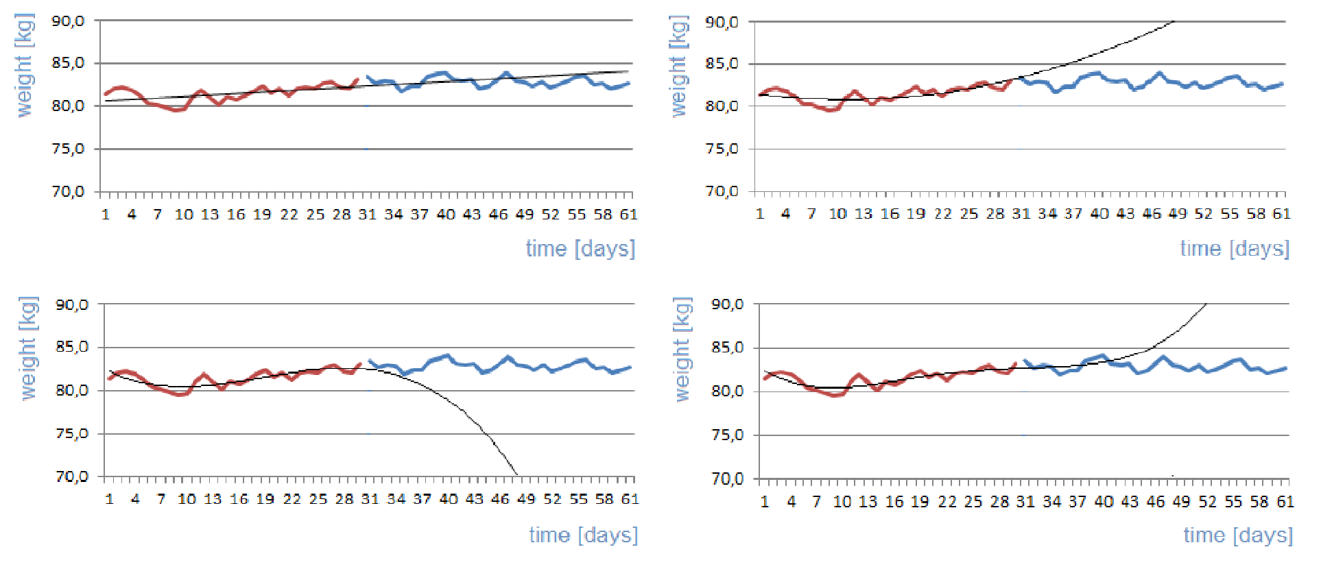
Figure 9.3 Polynomial approximation of a time series of body mass values (the approximation is based on values in the left half of the time series) – top left: linear approximation; top right: second-order polynomial approximation; bottom left: third-order polynomial approximation; bottom right: fourthorder polynomial approximation.
Chapter 9: Parametric decomposition of time series
9.1 Introduction
In the preceding chapters, we got acquainted with the concepts of time series decomposition to harmonic components. These concepts make possible to obtain useful information on characteristics of a time series and on relations between the basic components of that time series. The advantage of these procedures is the possibility of obtaining some knowledge of a time series without an a priori information about the event of interest. Unfortunately, results obtained in this way reflect the non-existence of information on the problem to be solved. For example, we got acquainted with artefacts that are introduced into the results of Fourier spectral analysis by the fact that periods of harmonic sequences do not correspond to the duration of recording and to the sampling period. And if we do not have a basic knowledge of frequencies of harmonic components of a time series, then the selection of an appropriate duration of recording is a lottery rather than a reasonably justifiable process. There are procedures that make the estimates of frequency spectra more specific by suppressing random artefacts, and there are also tests for the importance of individual spectral peaks; these processes, however, are beyond the scope of this text. Nevertheless, even an error-prone spectral estimate can serve as a good starting point for subsequent analyses or even for the development of models.
In some applications (related to medicine, biology, ecology, economics, meteorology, ...), events of interests are subject to external periodic influences (yearly, monthly, daily – both natural and human-made), which are obviously reflected in the observed time series. The connection of natural environmental influences therefore provides important information about the components of a time series; this information can subsequently be used in the development of a model of that time series.
The basic heuristic concepts of the composition of a time series were already mentioned in Chapter 1, where the additive and multiplicative (Figure 9.1) models of composition of a time series were introduced (Eqs. (1.2) and (1.3) in the form with a reduced argument):
x(n) = r(n) + z(n) + s(n) + ν(n)
and
x(n) = r(n).z(n).s(n).ν(n).
Let us repeat that r(n) represents a monotonic trend of a time series, z(n) stands for a longterm repetitive component with a period significantly longer than the duration of monitoring of the time series, s(n) is the oscillatory seasonal component, the period of which is shorter than the duration of the time series record, and ν(n) is the noise component. It is usually expected that the noise component represents the so-called white noise with a normal distribution, a zero mean value and a unit variance. The combination of trend together with long-term oscillation is often called a drift.
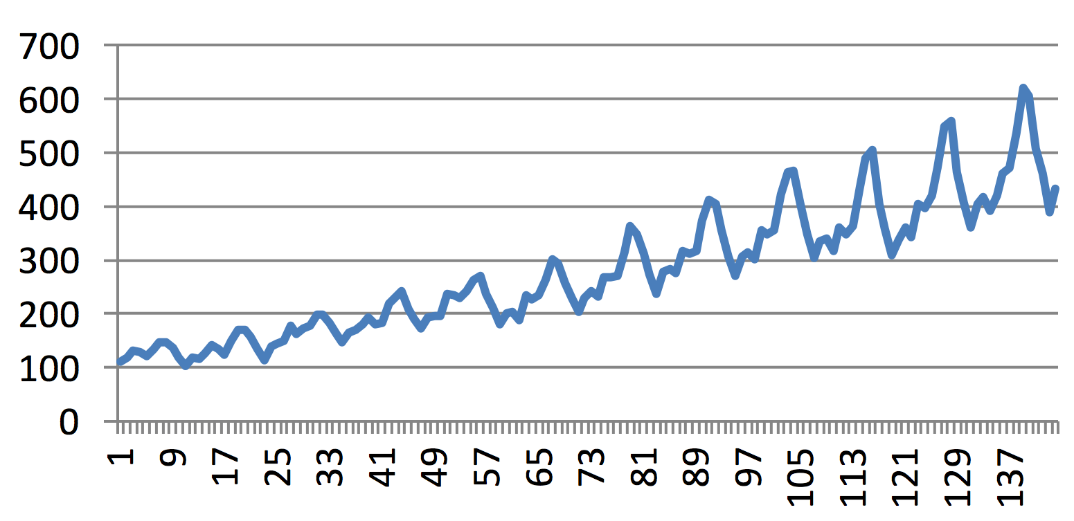
Figure 9.1 A typical trend in the development of the number of passengers travelling with one of American airline companies (with a monthly sampling) is shown here as an example of multiplicative dependence between the continuous increase in the number of passengers and seasonal changes in the number of passengers that occur each year: the magnitude of seasonal changes grows with the increasing number of passengers.
The significance of the above-mentioned components may vary in different problems to be solved. The decomposition of a time series, i.e. the separation of the significant component from all other components, is the fundamental task to solve a given problem. Any information, any characteristics of significant components apart from the rest of the time series, is needed to decompose a time series successfully. These characteristics are subsequently used for the construction of its mathematical model or even the model of the remaining components of a given time series. And finally, these models allow us to design and to run a separation algorithm. Individual components of a time series can differ in frequency characteristics, the distribution of values, the occurrence of specific graphoelements, etc.
Note
When considering both models of time series composition (the additive model versus the multiplicative model), the additive model is usually handier to use because linear algorithms can be used for the separation (for example, if individual components differ in frequency contents), as opposed to the multiplicative model. For this reason, the multiplicative model is often converted to the additive model by taking the logarithm of the time series (using the logarithm of any base). Based on this assumption, we can undoubtedly write ln[x(n)] = ln[r(n)] + ln[z(n)] + ln[s(n)] + ln[ν(n)]. However, before applying this transformation, it is essential to realise what potential consequences it could have on the characteristics of the time series as a whole and on the characteristics of its components – and whether it is possible and reasonable to tolerate such a change. For example, changes in the distribution of values and in spectral characteristics can be expected (Figure 9.2). It is also worth considering whether the logarithmic transformation of data (in cases where it is really essential) must be applied right at the start of time series processing or whether it might be applied after the separation of its components. In Figure 9.1, for example, separating the drift from seasonal changes (using a linear filter) should not be an issue because both components can easily be distinguished based on their frequency characteristics. After taking the log, however, frequency filtering would be out of the question due to frequency changes caused by the transformation. The dimension of individual components of the model is another fact to be taken into account when considering the application of the multiplicative model. All components of the additive model have the same dimension (i.e. they are expressed in the same units), whereas the multiplicative
model only permits one component (usually the drift) to have the same units as those of the time series as a whole. The remaining components of the model can only be expressed in relative dimensionless measures, which makes one think about their interpretation.
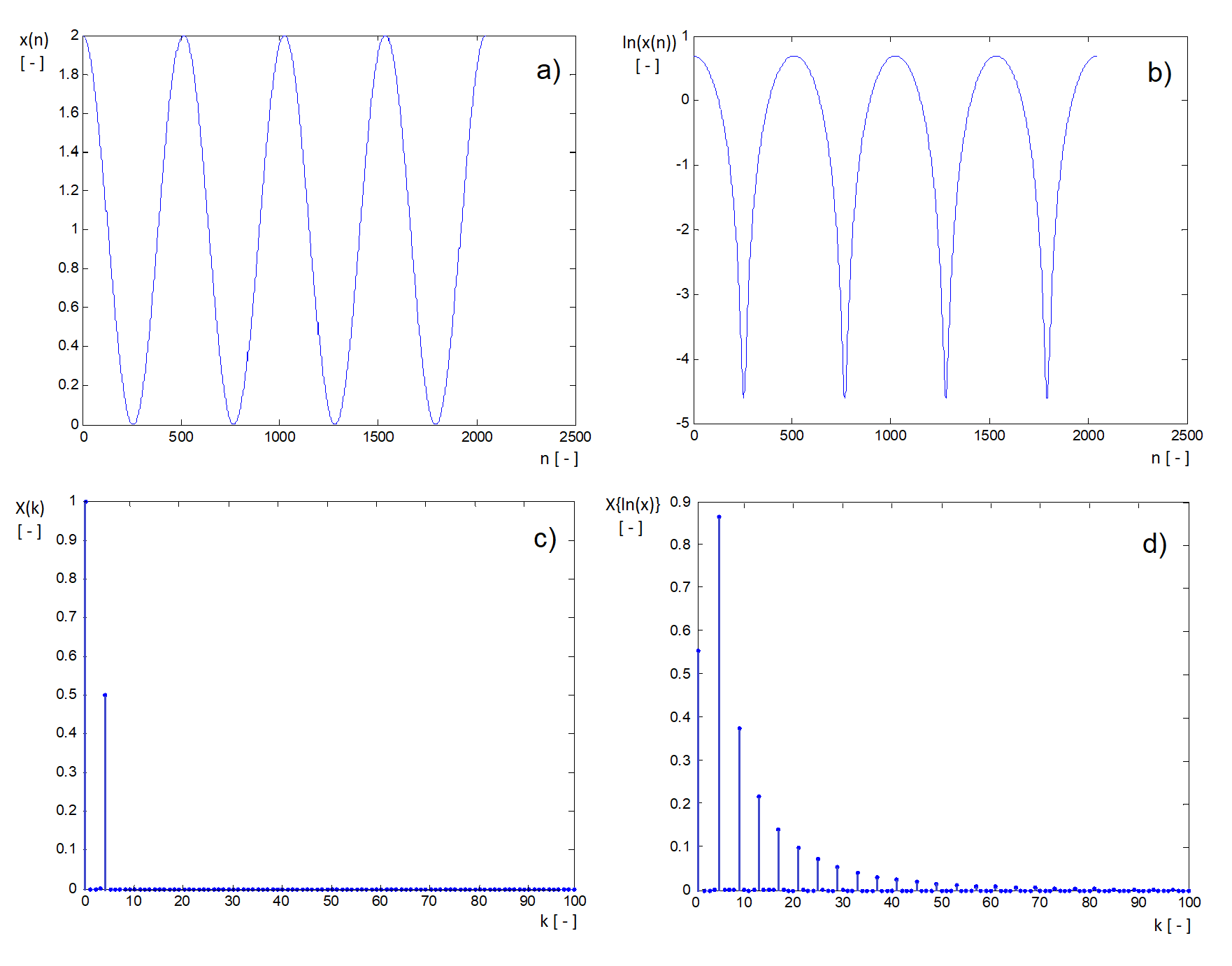
Figure 9.2 The effect of taking the logarithm of a harmonic sequence in the time domain and in the spectral domain – a) shape of the sequence x(n) = 1+cos(4π.10-3n); b) shape of the sequence ln[x(n)] (it can be easily found that function values of the first sequence fall within the interval < 0; 2 > , whereas in the second case, they fall within the interval (-ꝏ; ln2 > ); c) the frequency spectrum of the original sequence (there are only two components in the shown interval: a direct current component and a component corresponding to the harmonic waveform); d) the frequency spectrum of the sequence ln[x(n)] – in accordance with the change in sequence shape, the spectrum became more extended (in real sequences, whose components do not have an ideal harmonic form, such an extension can result into spectral overlaps, making impossible to use linear frequency filters).
9.2 Separating the trend/drit of a time series
Both the trend and the drift of a time series represent its slowly changing components. In principle, methods for the estimation of these components can be divided into two categories:
a) approximation by a specific sequence/function;
b) frequency filtering, based on filters such as low-pass filter etc.
Ad a)
In this case, we must decide about the type and order of the sequence to be used for the approximation of the slowly changing component, as well as about the way of estimating the parameters of its model. Using polynomial or exponential sequences is a common way of approximating and subsequently eliminating the slowly changing component of a time series. The character of the chosen approximating sequence should reflect the essence of the process to be described. Therefore, if a process determining the waveform of the slow component of a time series can be described by a linear model, it is natural to use some form of exponential sequence for its approximation (see Chapter 7). In cases of polynomial approximations (of any order), the estimation of their parameters is somewhat easier. Therefore, their application is often justified by computational demands rather than the effort to express the essence of the process that determines the course of a time series.
Note
When using a polynomial approximation, it might happen that the approximating sequence crosses the zero, although samples of a given time series really cannot take on other than nonnegative values. (Such time series are common in epidemiology, demography, etc.) To prevent this happening, a simple polynomial (usually linear) estimate of the course of a time series is often used for a growing trend, and an exponential sequence is used for the approximation of a decreasing time series. It means that a time series (or rather its trend component) is described by two different mathematical models. The question is to what extent is this approach – based on mathematical grounds rather than on the effort to capture the essence of the modelled process– justified.
Ad b)
There are many ways of designing a suitable linear model representing the slow component of a time series. Information about frequency characteristics of not only the drift, but also of other components of the time series, is essential for such a design. The decision about the computational structure of the model is important, too. Computations based on moving average (MA) are often used to estimate (or to eliminate) the drift. As shown in Chapter 8, this structure is suitable especially in cases where the low-frequency component of data has a relatively wide frequency band. On the other hand, autoregressive (AR) computational scheme is more suitable for a narrowband low-frequency component; moreover, the computation of its parameters is usually easier. A combination of both computational schemes gives the ARMA-type model. In connection with the effort to remove the drift from a time series (because drift is one of the important reasons of a time series non-stationarity), the ARIMA-type model is often introduced, where the inserted letter “I” represents the “integration” (AutoRegressive Integrated Moving Average). In formal terms, this computational structure is better for the description of individual component processes contributing to the final shape of a time series. However, frequency characteristics of a time series model can also be expressed by simpler, above-mentioned types of models. This chapter deals with approximation methods; see Chapter 10 for linear filtering methods.
9.3 Polynomial approximation
Polynomial approximation consists in the replacement of the slow component of a time series by a polynomial of a given order. Parameters of the approximating polynomial sequence are determined by a specific procedure of regression analysis. If the approximating sequence is a linear function of parameters/coefficients, a relatively simple method of least squares is sufficient. This method determines coefficients of the polynomial in such way that squared deviations of the approximating sequence from experimental values of the time series are minimised.
9.3.1 Linear trend
Leaving aside the “constant” trend r(n) = k0, where the constant k0 is given by the arithmetic mean of time series values, a linear function provides the simplest estimate of a time series trend. It is defined by
Let us suppose that values of the time series xn can be approximated by a line r(n) = k0 + k1n, where k0 and k1 are unknown coefficients that can be determined from the condition
The total squared deviation will reach its minimum if the following will hold for the optimal coefficients k0* and k1*:
If we determine partial derivatives according to Eq. (9.3), we get
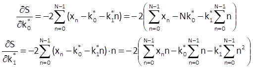
After substitution into Eq. (9.3), we get the following equations:

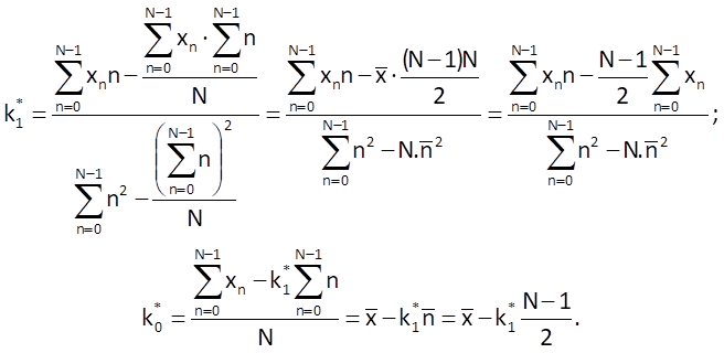
The solution of these equations provides formulas allowing us to determine the values of coefficients k0 and k1 for a straight line which optimally approximates the time series values:
If we use the linear trend model to predict the Mth value of a time series xpM , we get
9.3.2 Quadratic trend/drift
The following holds for a quadratic trend estimate:
and the defining system of equations to determine the optimal values of coefficients is
As a consequence, we can write the following for coefficients of this model:
where Δ = N.(Σ2Σ4 – Σ32) + Σ1(Σ2Σ3 – Σ1Σ4) +Σ2(Σ1Σ3 – Σ22) .
Finally, we can determine the predicted value of the Mth sample xpM by
Note
When solving problems in practice, it is usually not convenient to use higher-order polynomials, especially if it is necessary to use the developed model for the prediction of time series values. With regard to the computation of optimum values of coefficients, the computational complexity grows tremendously for higher-order polynomials, as shown by the comparison of computational complexity in the three above-mentioned cases. Moreover, although the approximation by higher-order polynomials is more accurate within a known interval, it is significantly less reliable beyond this interval, as shown in Figure 9.3.
Figure 9.3 Polynomial approximation of a time series of body mass values (the approximation is based on values in the left half of the time series) – top left: linear approximation; top right: second-order polynomial approximation; bottom left: third-order polynomial approximation; bottom right: fourthorder polynomial approximation.
9.4 Exponential approximation
9.4.1 Simple exponential trend approximation
In this case, the approximating sequence is given by
If k0 is non-negative, then the sequence r(n) is increasing for k1 > 1 and decreasing for k1 ∈ (0; 1). For a negative k1, the sequence r(n) loses its monotonicity: depending on the value of k1, the sequence retains its increasing or decreasing trend but its values oscillate with a changing polarity.
A sequence defined in this way has a shape given by the solution of a first-order linear differential equation:
where ρ is the so-called growth coefficient. The solution of this equation can be written as
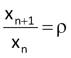
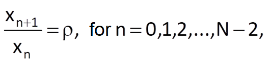
where x0 is the initial condition. If we compare Eq. (9.12) with the solution indicated in Eq. (9.14), we can state that the initial condition x0 corresponds to the coefficient k0 and that the growth coefficient ρ corresponds to the coefficient k1. Furthermore, if we divide Eq. (9.13) by xn, we get the formula for a ratio of two neighbouring samples of solution; this ratio is constant and is equal to the growth coefficient, i.e.
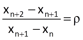
A similar formula also holds for the ratio of two neighbouring first differences, which is again constant and is equal to the growth coefficient ρ, i.e.
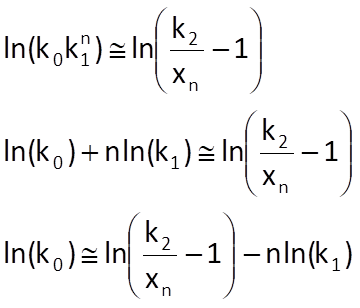
If we wanted to use the method of least squares again to determine the optimum values of coefficients k0 and k1, our effort would be complicated by a multiplicative (i.e. non-linear) dependence of both coefficients, as shown in Eq. (9.12). For this reason, the defining system of equations to determine coefficients k0 and k1 would not be linear, which would have unpleasant consequences. Therefore, an attempt to transform a non-linear equation (namely Eq. (9.12)) to a linear equation seems to be more convenient. In this case, we can achieve this by taking the logarithm of the original formula, which results into
a similar form as that seen in Eq. (9.1) for a linear trend. Values of ln[k0*] a ln[k1*] (and therefore also values of k0* a k1*) can be then determined using a procedure similar to the above-mentioned one.
However, using the logarithm, has all the disadvantages mentioned in Section 9.1. The distribution of values (and therefore their mean value) will change, and the distribution of errors will change, as well – from the normal distribution to the log-normal distribution. All these changes can have an impact on the optimality of approximation. The impact of taking the logarithm can be partly rectified by weighting individual terms of the minimised expression. For the original exponential function, we can write
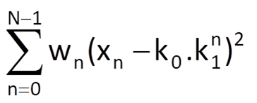
where wn are the applied weighting coefficients. However, after taking the logarithm, , we are going to minimise the expression
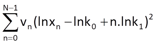
where weighting coefficients vn should be determined in a way which would lead to approximately the same estimates of coefficients k0 and k1 in both cases. It can be established for the applied logarithmic function (beyond the scope of this textbook) that equivalent values of parameters k0 and k1 can be obtained if the weights are selected as follows:
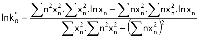
If we do not prefer any value of a given time series during the computation (i.e. in cases where all weights wn are equal, ideally wn = 1, for all values of the index n), we get the following formula for the values of transformed weights:
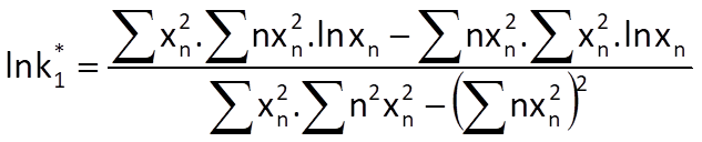
Optimal values of coefficients k0 and k1 for these weights can then be computed by the following formulas:
and
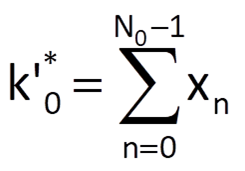
Both coefficients can be determined partly heuristically (and not quite optimally) based on the equivalence of Eqs. (9.12) and (9.14) and by using Eq. (9.15). Because the coefficient k0 represents the initial value of the exponential sequence approximating the time series trend, we will estimate its value as the arithmetic mean of the first N0 values of a given time series, where the number N0 depends on the characteristics of that time series. Then, it follows that
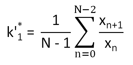
After that, we will estimate the coefficient k1 using Eq. (9.15) by an optimal fitting of ratios
by a constant. In the case, we get
The predicted value of the Mth sample xpM is then determined by a formula
9.4.2 Exponential trend with a limitation
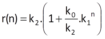
In this case, the approximating sequence is given by
or, alternatively, by
Optimal values of coefficients k0, k1 a k2 can only be determined by a system of non-linear equations or, not so optimally, by means of some heuristic algorithm.
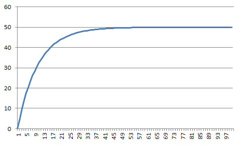
Figure 9.4 Example of implementation of an exponential sequence according to Eq. (9.26a) with parameters k0 = -50, k1 = 0.9, and k2 = 50.
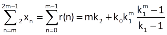
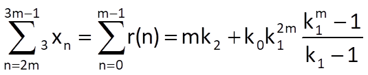
One of the possible heuristic algorithms divides the approximated time series into three equally long segments with a length of m samples. Provided that the sum of deviations of the approximating sequence from the measured values is equal to zero in each segment, we can write the following (based on the formula for the sum of a finite geometric series):
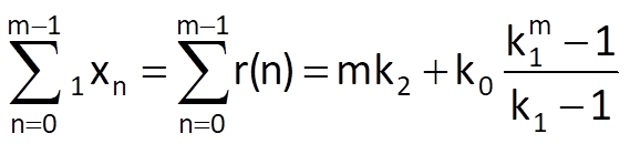
Likewise, we get the following formulas for the second segment and the third segment, respectively:
Then we can apply the elimination method on these three equations in order to determine pseudo-optimal values of all the three coefficients, for example:
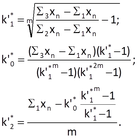
Then, the predicted value of the Mth sample xpM can be determined by
9.4.3 Logistic trend approximation
The logistic sequence (a sigmoid function) is again defined by a formula with three parameters:
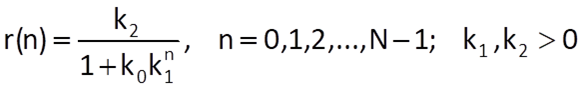
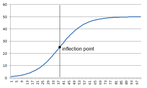
Figure 9.5 Example of implementation of a logistic sequence according to Eq. (9.30) with parameters k0 = 50, k1 = 0,9 and k2 = 50 and an inflection point for n 37
This way of approximation respects the characteristics of many real processes that are limited from both sides, such as the blood pressure, body height, substance concentration etc. The logistic function must have an inflection point in order to be able to achieve a limitation at both sides; this inflection point is located at n = -ln(k0)/ln(k1). The derivative of the logistic function (provided that the variable n is continuous), which is given by
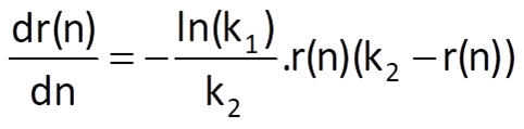
is symmetric about the inflection point.
The parameters k0, k1 and k2 are usually estimated by various pseudo-optimal procedures.
Because the defining equation for the logistic trend can be almost thought of as the inversion of the exponential trend with a limitation, it is possible to use the procedure employed in the preceding Section 9.4.2 on the time series with reciprocals, i.e. 1/xn. Eq. (9.30) then needs to be converted to the form
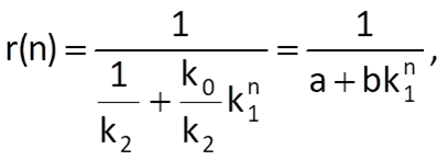
where a = 1/k2 and b = k0/k2. Then, as was the case with Eq. (9.28), we can write
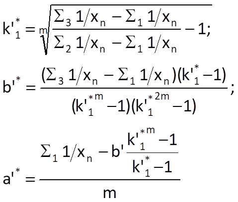
and, subsequently, we get k’2* = 1/a’* and k’0* = a’*.b’*. The so-called difference estimate is the second possible way of estimating the optimal values of parameters. If we use a difference instead of the derivative in Eq. (9.31) and substitute time series values xn for the values of trend sequence r(n), we get
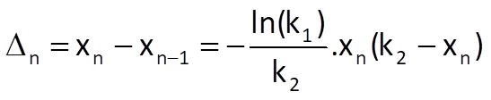
and therefore
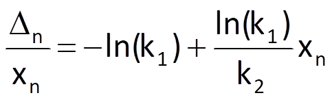
which, from a view point of parameters –ln(k1) and ln(k1)/k2, represents a linear approximating sequence and its parameters; the values of k’1* a k’2* can be subsequently determined in a standard way, i.e. by the method of least squares.
To determine the optimal value of the last necessary parameter k0, we will again substitute real time series values xn for trend values r(n) in Eq. (9.30); we will then convert this equation to the form
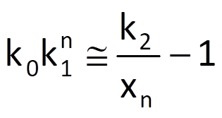
We can subsequently write
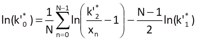
If we add up the obtained formula for all n= 0,1,2,…,N-1, we finally get the equation for the computation of k’0*or, more precisely, its logarithm:
9.4.4 Gompertz trend approximation
As it was the case with the logistic trend, the approximating sequence defined by
or, alternatively, by
has the characteristics of a sequence limited from both sides. Unlike the logistic trend, however, its first derivative (provided that n is continuous) is not symmetric about any inflection point.
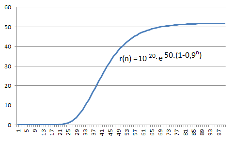
Figure 9.6 Example of implementation of a Gompertz sequence according to Eq. (9.38b).
The optimal values of parameters k0, k1 and k2 can be estimated by the same procedure as that used in case of the exponential trend approximation with a limitation (see Section 9.4.2); the only difference is that we will use logarithms of time series values rather than the values themselves.