Time Series Jiří Holčík
Harmonic sequence is one of the basic periodic sequences. Its shape is defined by trigonometric functions sin(α) [1] or cos(α) . With respect to context explained further in the text, a decision has to be made now which of the two functions will be thought of as the reference function. Let us therefore decide (and there are several good reasons for this decision) that from now on, a harmonic sequence defined by the following formula will be considered a reference sequence:
where A is a positive real constant, the so-called amplitude [2] of a harmonic sequence (this constant has the same units as the variable represented by the harmonic sequence), and Ω is also a positive real constant, the so-called angular frequency [3] (expressed as the angular displacement per unit time, e.g. in rad/s). The angular frequency is responsible for changes in time scale (as already mentioned in Chapter 2.3.2). Finally, ϕ0 is again a real constant, the so-called initial phase. The initial phase determines the time shift of harmonic sequence against the origin, i.e. for nTs = 0. This interpretation follows from transcription of the above-mentioned definition to the form
where n0 = -ϕ0/ΩTs [4]. Introduction of the initial phase simplifies the description of real data by a harmonic sequence because the start of recording real data usually does not correspond to the origin of time axis of the cosine function. The argument α of the defined sequence determines the value of its phase.
The fundamental period and the fundamental angular frequency are linked to frequency f of a harmonic sequence, which is given by
If angular frequency is expressed in radians per unit time, the fundamental period of a harmonic sequence is given by
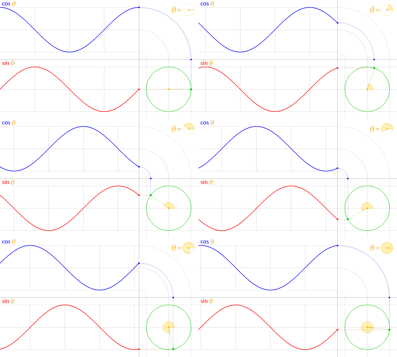
This equation implies that in discrete sequences, the angular frequency is tightly linked to the sampling period (or the sampling frequency); furthermore, it implies that the angle 2π [rad] corresponds to the period T (Figure 2.7).
Figure 2.7 Circular motion of a point projected to a time axis. By LucasVB (Own work) [Public domain], via Wikimedia Commons
Example:
Figure 2.8 shows the harmonic sequence x(nTs) = A.cos(ΩnTs + ϕ0) for A=1, ϕ0 = 0 and angular frequency Ω for (a) T = 8Ts or (b) T = 4T’s. If we had T’s = 2Ts, then the angular frequency Ω would be the same in both cases (as shown in the Figure). However, if we had T’s = Ts, then the angular frequency would increase twofold. This example demonstrates that a ratio of angular frequencies (or of sampling periods), rather than their absolute values, are important to display values of a harmonic sequence (or any periodic sequence in general). This fact is one of the reasons why the time scale is suppressed in the formal notation of values of discrete sequences, and a notation according to Eq. (2.2) is usually used instead.
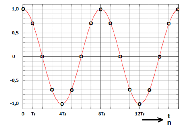
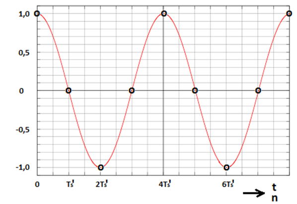
Figure 2.8 Values of harmonic frequencies for A = 1, ϕ0 = 0 , and angular frequency Ω for (a) T = 8Ts and (b) T = 4T’s provided that T’s = 2Ts.
The above-mentioned example illustrates one more fact. The periodicity of discrete sequences is related to the ratio of period of the sampled variable and the sampling period. It is obvious that a sampled continuous periodic variable with a period T is represented by a periodic discrete sequence with the same period only if the period T is just equal to an integer N multiple of the sampling period, i.e. if T = NTs. If this is not the case, the period of a discrete sequence is increased depending on the decimal part after the division T/Ts. If the decimal part of the division is equal to 0.5 (Figure 2.9), the period increases twofold; if the decimal part is equal to 0.33…, the period increases threefold, etc. If the ratio of both periods (T/Ts) is an irrational number, then the resulting sequence is non-periodic, even though the original variable is periodic.

Figure 2.9 Change of periodicity for a variable after sampling with a sampling period which did not correspond to a zero-remainder integer division of T / Ts (decimal part of the division was equal to 0.5).
Chapter 2: Basic types of discrete variable models and mathematical operations on them
2.1 Introduction
2.1.1 One assumption to start with
Discretisation of a continuous function leads to the fact that values of that function are only known in specified points in time.
Sampling has caused the conversion x(t) → x(nTs) . This notation still suggests that even a discrete sequence depends on time. However, the sampling period is a constant; therefore, samples of discrete sequences are often shortly denoted as x(n) or xn in scientific literature. The advantage of this way of notation is that it is not linked to time as an independent variable, that it can be used for time series as well as for the description of digital images, for example in the form x(n,m). On the other hand, this advantage can be a disadvantage at the same time, namely when attempting to explain some other relations, such as the conversion of a sequence from the primary time representation to a frequency representation, as we will see later. In the following text, we will prefer the notation respecting the time dependence of data (because it is useful to keep in mind that there is time dependence). We will use the shorter notation of the argument where no problems would be expected.
2.2 Basic unary operations on sequences
2.2.1 Multiplication by a constant
Multiplying the function by a constant A will increase (decrease) the instantaneous value of the function A-times. For A > 1, we say that there has been an amplification; for A < 1, this is called an attenuation (Figure 2.1).
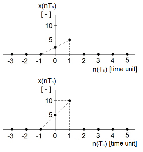
Figure 2.1 Multiplication by a constant: A = 2
2.2.2 Change of time scale
Multiplying the independent variable (time) by a constant k changes the time scale x(nkTs). Because the constant is a real, non-integer number in general, changing the sampling period is formally used to change the time scale in a time series (Figure 2.2). For k < 1, the sampling period gets shorter and the time axis compresses. For k > 1, the sampling period gets longer and the time axis expands.
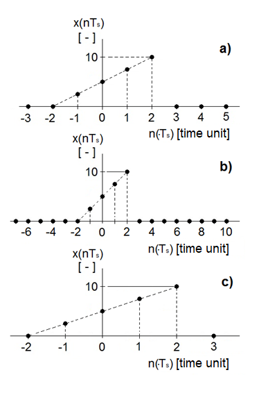
Figure 2.2 Change of time scale: (a) original; (b) k = 2; (c) k = 2/3
2.2.3 Time shift
Adding a value n0 (where n0 is an integer) to the original position n of a sample in time shifts the time series to the left along the time axis. Similarly, subtracting a value n0 (where n0 is an integer again) from the original position n of a sample in time shifts the time series to the right along the time axis. In other words, a sequence is shifted back by adding a value n0, and it is shifted ahead by subtracting a value n0 (Figure 2.3).
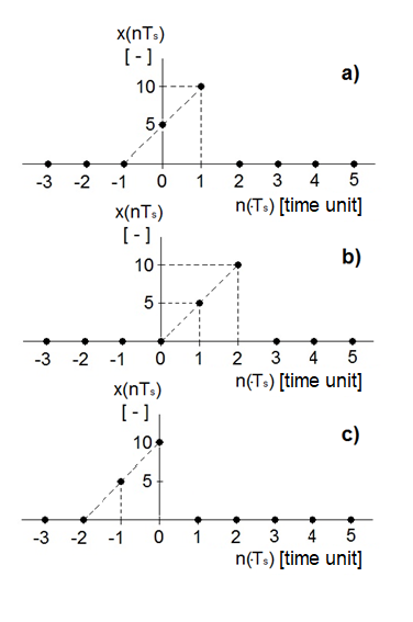
Figure 2.3 Time shift: (a) original x(n); (b) sequence x(n-1); (c) sequence x(n+1)
2.2.4 Inversion of time axis
Changing the sign of time argument leads to the inversion of time axis. If time shift is required at the same time, the sign must be changed in all terms of the argument (Figure 2.4).

Figure 2.4 Inversion of time axis: (a) original x(n); (b) sequence x(-n); (c) sequence x(-n-1)
2.3 Periodic sequences
2.3.1 Introduction
The basic criterion for distinguishing between two basic types of time series models consists in the question whether the course of a time series is repeated in time, i.e. whether it is ideally periodic or not.
Definition 2.1
A sequence x(nTs) is periodic with a period T = NTs if and only if the following condition holds:
or, in a simplified form of the argument (this is only possible for regular sampling):
The smallest value of T or N (if such a value exists) satisfying Eq. (2.1) or (2.2) is the fundamental period of the sequence.
All time series (sequences) not satisfying Eq. (2.1) or (2.2) are non-periodic.
Example:
A periodic time series can be defined by the following equation, for example:

Figure 2.5 Periodic sequence according to Eq. (2.3)
Please note that periodic sequences are ideal mathematical models. The course of real variables, even though it is repeated, is usually not exactly periodic (see Figure 2.6, for example). We usually use the term repetitive variables in these cases.
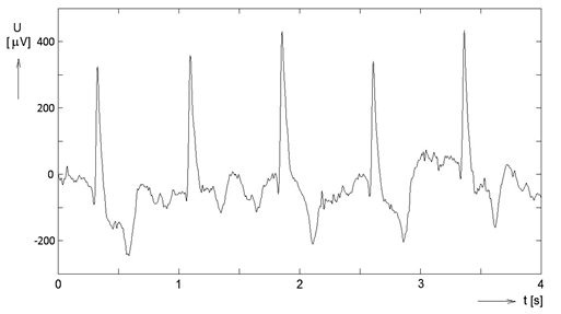
Figure 2.6 ECG signal of a horse in gait. Even though the electrical activity of the heart is repeated, the ECG signal is different in each cardiac cycle.
2.3.2 Harmonic sequence
Basic terms
Harmonic sequence is one of the basic periodic sequences. Its shape is defined by trigonometric functions sin(α) [1] or cos(α) . With respect to context explained further in the text, a decision has to be made now which of the two functions will be thought of as the reference function. Let us therefore decide (and there are several good reasons for this decision) that from now on, a harmonic sequence defined by the following formula will be considered a reference sequence:
where A is a positive real constant, the so-called amplitude [2] of a harmonic sequence (this constant has the same units as the variable represented by the harmonic sequence), and Ω is also a positive real constant, the so-called angular frequency [3] (expressed as the angular displacement per unit time, e.g. in rad/s). The angular frequency is responsible for changes in time scale (as already mentioned in Chapter 2.3.2). Finally, ϕ0 is again a real constant, the so-called initial phase. The initial phase determines the time shift of harmonic sequence against the origin, i.e. for nTs = 0. This interpretation follows from transcription of the above-mentioned definition to the form
where n0 = -ϕ0/ΩTs [4]. Introduction of the initial phase simplifies the description of real data by a harmonic sequence because the start of recording real data usually does not correspond to the origin of time axis of the cosine function. The argument α of the defined sequence determines the value of its phase.
The fundamental period and the fundamental angular frequency are linked to frequency f of a harmonic sequence, which is given by
If angular frequency is expressed in radians per unit time, the fundamental period of a harmonic sequence is given by
This equation implies that in discrete sequences, the angular frequency is tightly linked to the sampling period (or the sampling frequency); furthermore, it implies that the angle 2π [rad] corresponds to the period T (Figure 2.7).
Figure 2.7 Circular motion of a point projected to a time axis. By LucasVB (Own work) [Public domain], via Wikimedia Commons
Example:
Figure 2.8 shows the harmonic sequence x(nTs) = A.cos(ΩnTs + ϕ0) for A=1, ϕ0 = 0 and angular frequency Ω for (a) T = 8Ts or (b) T = 4T’s. If we had T’s = 2Ts, then the angular frequency Ω would be the same in both cases (as shown in the Figure). However, if we had T’s = Ts, then the angular frequency would increase twofold. This example demonstrates that a ratio of angular frequencies (or of sampling periods), rather than their absolute values, are important to display values of a harmonic sequence (or any periodic sequence in general). This fact is one of the reasons why the time scale is suppressed in the formal notation of values of discrete sequences, and a notation according to Eq. (2.2) is usually used instead.


Figure 2.8 Values of harmonic frequencies for A = 1, ϕ0 = 0 , and angular frequency Ω for (a) T = 8Ts and (b) T = 4T’s provided that T’s = 2Ts.
The above-mentioned example illustrates one more fact. The periodicity of discrete sequences is related to the ratio of period of the sampled variable and the sampling period. It is obvious that a sampled continuous periodic variable with a period T is represented by a periodic discrete sequence with the same period only if the period T is just equal to an integer N multiple of the sampling period, i.e. if T = NTs. If this is not the case, the period of a discrete sequence is increased depending on the decimal part after the division T/Ts. If the decimal part of the division is equal to 0.5 (Figure 2.9), the period increases twofold; if the decimal part is equal to 0.33…, the period increases threefold, etc. If the ratio of both periods (T/Ts) is an irrational number, then the resulting sequence is non-periodic, even though the original variable is periodic.

Figure 2.9 Change of periodicity for a variable after sampling with a sampling period which did not correspond to a zero-remainder integer division of T / Ts (decimal part of the division was equal to 0.5).
Why harmonic sequence?
The reasons why it is useful to consider the harmonic shape to be the basic model of periodic movement are historical, physical, geometric and computational, although the latter ones are at the same time one reason to avoid it. In fact, this model requires a relatively high level of accuracy in order to express individual values.
Physical reasons are related to various forms of movement. A harmonic function can be used to describe the movement of a pendulum, the oscillation of a spring (if the displacement is small), the oscillation of a string (hence the musical origin of its name) or the motion of a point on the circumference of a circle (Figure 2.7). Moreover, the latter association provides not only a visual explanation of all three parameters used in Eq. (2.4), but also instructions to other forms of mathematical description of the harmonic function (or the harmonic sequence). The amplitude A is determined by the radius of the rotating circle, the angular frequency Ω is linked to the rate of rotation, and the initial phase ϕ0 determines the initial point on the phase circle.
One interesting property of the harmonic function is that the sum of two harmonic functions with the same angular frequencies provides a harmonic function with the same frequency.
The behaviour of harmonic functions during sampling is another important feature to keep in mind. With a sampling period Ts, harmonic sequences A.cos(ΩnTs + ϕ0) a A.cos(Ω‘nTs + ϕ0) have the same behaviour if the difference of angular frequencies Ω - Ω‘ is equal to an integer multiple of the sampling frequency, i.e. fs = 1/Ts.
Other forms of expressing the harmonic sequence
The so-called trigonometric form of a harmonic sequence is A1cos(ΩnTs) + A2sin(ΩnTs). Therefore, the following equation must be valid:
Example:
Prove that the trigonometric form of harmonic sequence is valid.
Solution:
If we use the trigonometric formula for the cosine of sum of two angles, according to which
we will get
A.cos(ΩnTs + ϕ0 ) = A.cos(ΩnTs).cos ϕ0 - A.sin(ΩnTs).sinϕ0 = A.cosϕ0.cos(ΩnTs) - A.sin ϕ0.sin(ΩnTs).
Therefore,
Then, after determining the second power of both the parts of Eq. (2.11) and summing them, we will obtain
Because cos2α + sin2α = 1, the amplitude A can be expressed as
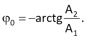
The initial phase ϕ0 is obtained by dividing both parts of Eq. (2.11)

Finally, we get
Example:
Determine the sum of two harmonic sequences with the same angular frequency and different initial phase, i.e.
x(nTs) = A1.cos(ΩnTs + ϕ01) + A2.cos(ΩnTs + ϕ02).
Solution:
Again, by using the equation for the cosine of sum of two angles (see the preceding example), we get:

which resulted into the trigonometric form of a harmonic sequence and, based on the conclusions from the preceding example, we get

As it follows from Eq. (2.4), the waveform of a harmonic sequence is unambiguously determined by values of three parameters – the amplitude A, the angular frequency Ω and the initial phase ϕ0 – for all points in time. Apart from a time dependency, the properties of a harmonic sequence might therefore be graphically expressed by mutual relations of these parameters, usually displayed in two planes: (1) amplitude versus angular frequency (or frequency), (2) initial phase versus angular frequency (or frequency). As we will see later in the text, this concept of displaying the properties of a harmonic sequence depending on its frequency can be used to draw the spectrum of a discrete sequence (time series). In the meantime, keep in mind that the frequency spectrum of a sequence (time series) repre-sents the distribution of amplitudes and initial phases of individual harmonic components of the time series, depending on its frequency. Although a harmonic sequence is defined by Eq. (2.4), it can be also described by other means, following from the Euler’s formulas
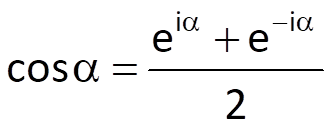
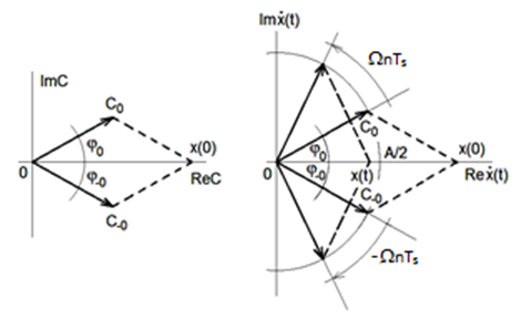
Figure 2.10 Complex amplitudes of exponential components of a harmonic sequence; temporal dynamics of exponential components of a harmonic sequence
This approach is used more frequently because the complex exponential function eiα can be manipulated more easily (under certain circumstances) than the traditional trigonometric functions sinα a cosα.
Multiplying the first equation by 2, the second equation by 2i and summing up the results gives
It means that the course of a harmonic sequence defined by Eq. (2.4) can be also expressed as the real part of a complex function eiα, i.e.
which corresponds to the projection of a circular motion represented by the movement of head of the vector A.exp[i(ΩnTs+ ϕ0)] in the complex plane to the real axis (Figure 2.10).
Because the cosine function is even, the following holds:
where ẋ*(nTs) is the complex conjugate of ẋ(nTs). Eq. (2.21) has introduced the negative angular frequency, which can be geometrically interpreted (physical interpretation would be rather hard to find) by the angular velocity of rotation of vector A.exp[i(-ΩnTs– ϕ0)] in the opposite direction (clockwise) than in case of vector A.exp[i(ΩnTs+ ϕ0)].
Using Eq. (2.18) for cos(•), we get
If we denote
we get
This means that a harmonic sequence can be expressed by the sum of two complex conjugate expressions that are equal to instantaneous values of complex exponential functions describing the opposite rotation of heads of vectors Ċ0.eiΩnTs and Ċ-0.ei(-Ω)nTs in the complex plane (Figure 2.11). Therefore a harmonic sequence is again expressed by complex exponential functions, now as a sum of complex conjugates, but without the necessity of searching – often awkwardly – for the real value of the function given by Eq. (2.20).
2.4 Non-periodic sequences
2.4.1 One-shot sequences

Figure 2.11 Discrete representations of a unit impulse (left) and a unit step (right)
Definition 2.2
A discrete unit impulse is defined as

A discrete unit step is defined as

The following holds for a unit impulse

or

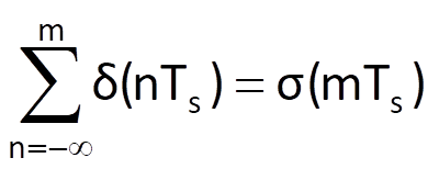
The mutual relation between the two one-shot sequences is determined by the two following equations:
and
A discrete unit rectangular impulse (Figure 2.14) with a length of N samples is defined by
It can be derived from a unit step, similarly to the unit impulse in Eq. (2.30), by
It means that from this point of view, a unit impulse can be understand as a unit rectangle with a length of 1.
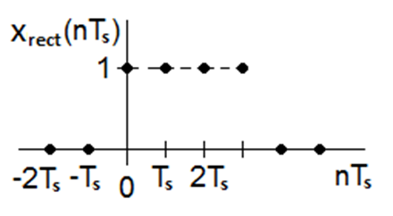
Figure 2.12 Discrete unit rectangular impulse with a length of 4
2.4.2 Random sequences
Random sequences represent another important type of non-periodic discrete sequences. They are considered to be the result of discrete random processes. Unlike the general term “process”, the random process is a mathematical abstraction that describes the probability characteristics of a specific source of data. It can be stated that a discrete random process represents the set of all occurrences of random sequences with specific characteristics.
In the signal theory, random sequences are often referred to as noise, whereas statistics uses the term variability, which is a bit more general. By definition, behaviour of random sequences cannot be exactly specified; these sequences can only be described by their general statistical properties or parameters. Probability distribution of random sequence values at each point in time is the most general description of random sequence behaviour. This concept then leads to a rather extreme idea that a deterministic sequence is a special case of random sequence with a unit probability of occurrence of the respective value (given by a deterministic rule).
The most frequently used abstraction is the so-called white noise, which is characterised by a normal distribution of function values a zero mean value, a defined variance and independent neighbouring values. The attribute “white” is based on the analogy with white light, which contains equally represented components of all wavelengths (or frequencies). Likewise, a white noise contains equally represented components of all frequencies.
When dealing with random processes and functions, there are two important terms to know: stationarity and ergodicity.
A stationary random process is a process whose form of behaviour (i.e., its probability structure, given by probability distribution, for example) is time-independent. In other words, any probability characteristics of a stationary process do not depend on the position of the time axis origin.
From the practical point of view, we often perceive the concept of stationarity in the broader sense of the term, when only first-order and second-order statistical moments, the mean value, the variance and the autocorrelation or autocovariance function/sequence are required not to change with the independent variable.
An ergodic random process is a process whose all realisations have the same probabilistic structure and the same probability characteristics. Its probability characteristics can then be estimated from a single (in fact, any) realisation of the random process.
We usually require the analysed process to be both stationary and ergodic because it is more convenient for a subsequent analysis. In general, however, an ergodic process does not necessarily have to be stationary and vice versa – although some definitions of the ergodic process also require it to be stationary.
2.5 Basic binary operations on sequences
Leaving aside the elementary operations such as the sum and product or other – for example logical – operations on binary sequences, convolution and correlation (or the computation of values of a correlation function) are thought of as the two basic operations to be applied on two discrete sequences.
2.5.1 Convolution
This chapter introduces the definition of convolution, some of its properties and algorithms for its computation. The practical importance of convolution will follow from chapters dealing with linear systems.
Definition 2.3
Convolution is a mathematical operation between two sequences x1(n) and x2(n) of the same argument, defined by

where sequence x2(n) is called the convolution kernel.
The sequence x(n), which is the result of convolution, can be thought of as the sequence x1(n) modified by characteristics of the convolution kernel (x2(n). As follows from the below-mentioned commutative law, the significance of both input sequences can be interchanged. The significance of the convolution can also be perceived otherwise – as the weighted mean of sequence x1(m) at time n, while weighting is given by sequence x2(-m) shifted by time n. Although the variable n is considered to be time in this context, it can be of any character in general.
The above-mentioned convolution formula is widely used not only in time series processing, but also in probability theory, statistics, computer vision and other disciplines.
The following rules hold for convolution:
- Commutative law:
- Distributive law:
- Associative law:
- Time-shift law
For causal sequences, i.e. sequences in which x(n) = 0 holds for n < 0, the convolution formula changes to

In real conditions, i.e. when processing real data, sequences x1(n) and x2(n) are obviously not infinite but have a finite length. Suppose there are N1 samples in general for sequence x1(n) and N2 samples for sequence x2(n). Furthermore, let x1(n) = 0 for (n < 0) Ʌ (n > N1-1) and, likewise, that x2(n) = 0 for (n < 0) Ʌ (n > N2-1). In that case, it is

The algorithm to compute the convolution of two finite sequences consists in the sum of partial products of elements of sequence x1 and elements of sequence x2, which is time-inverted and shifted by n elements in the positive direction of time axis (Figure 2.13).
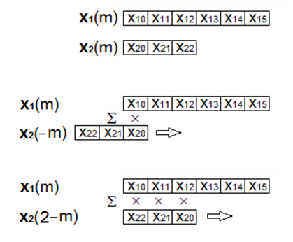
Figure 2.13 Diagram of the computational algorithm for the convolution of finite sequences.
Example:
Compute the convolution of sequences x1 = {x10, x11, … x13} and x2 = {x20, x21, x22}.
Solution:
Sometimes the following computational diagram is also used

Example:
Use the above-mentioned computational diagram to compute the convolution of two sequences x1(n) = {1, 2, -2, -1} and x2(n) = {1, -1, 1} (Figure 2.16).
Solution:
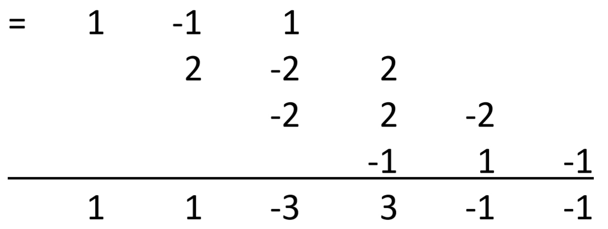
Therefore, the result of convolution of two sequences is the sequence x(n) = {1, 1, -3, 3, -1, -1} (Figure 2.14)..
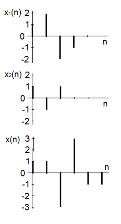
Figure 2.14 An example of convolution of two sequences (see the Example above)
Figure 2.13 and computational diagrams in preceding examples imply that the convolution sum at the beginning (but also at the end) of computation does not involve all partial products that it should duly involve, depending on the length of both sequences; thus, a certain transient event/process occurs.
This event could be eliminated provided that at least one from the two sequences is periodic.
Suppose that the length of both sequences is N and, at the same time, let N be also the period of sequence x2(n). Then the convolution can be defined as

Such way of computation is called a circular convolution and its computational diagram is shown in Figure 2.15.
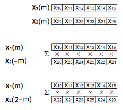
Figure 2.15 Computational diagram for a circular convolution
Width property of convolution
If the durations (widths, i.e. numbers of samples in a sequence that are different from zero) of sequences x1(n) and x2(n) are finite, for example N1 in case of sequence x1(n) and N2 for sequence x2(n), then the number of samples of the resulting convolution sequence is equal to N1 + N2 - 1 (see example based on Figure 2.14).
Convolution of a sequence with unit impulse
Convolution of a sequence x(n) with a unit impulse results in sequence x(n).
Definition of convolution implies that

Because δ(n-m) represents a unit impulse shifted from the origin by m samples, the sum in Eq. (2.41) is equal to the value of x(m) in m = n, i.e. x(n). Therefore,
Notes
1 The term sinus was already used in early 15 century, meaning “hollow curve or cavity in the body”. It is derived from Latin sinus, meaning “bend, fold, curve, a bent surface; a bay, bight, gulf; a fold in land,” but also “fold of the toga about the breast,” hence “bosom,” and figuratively “love, affection, intimacy; interior, inmost part;”. The word is of unknown origin.
2 amplitude (Latin amplitudo) – the “state or quality of being ample”
3 frequency (lat. frequentia) – the Latin word meant “an assembling in great numbers, a crowding; crowd, multitude, throng,” The sense in physics (“rate of recurrence”), especially of a vibration, is from 1831.
4 In this case, where the sequence is given by an equation, the constant does not necessarily have to be an integer.
