Time Series Jiří Holčík
Chapter 6: External (input-output) description of systems primarily in the frequency domain
6.1 Introduction
In the example at the end of the previous chapter, we used difference equations to describe the behaviour of a one-species population under different conditions. Difference equations represent the basic way of the so-called external (input-output) mathematical description of real systems which, based on the knowledge of values of the input sequence and system parameters, leads to the computation of output variable(s) – either analytically or numerically.
In case of a non-autonomous system, we can write the difference equation in its most general form as
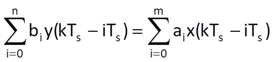
or alternatively, for a normalised sampling period, as

where ai and bi are system parameters, x(k) are values of the input sequence and y(k) are values of the output sequence. If the system is autonomous (i.e. without an input), the difference equation is homogeneous, with the right-hand side equal to zero.
In general, parameters ai and bi can be functions of both input and output variables (non-linear systems) and of time, too (time-variant systems). If the parameters are constant, the system meets the superposition principle and the system is linear. The value n determines the maximum delay for samples of the output sequence and the system order at the same time, whereas m determines the maximum delay for samples of the input sequence, which is involved in the calculation. An alternative notation of the difference equation has the form of expression for the computation of the kth output sample, which employs the value of the kth sample of input sequence and previous samples of both input and output sequences up to the delay m or n, respectively. The formula has the form

The above-mentioned recursive equation implies that if we want to compute the value of output for k = k0, we need to know not only the values of input samples from x(k0) to x(k0 – m), but also the values of output samples from y(k0 – 1) to y(k0 – n). The requirement on input data defines the minimum value of k0, i.e. k0 ≥ m. As regards the requirement on output data, the values of actually delayed output samples are not known at the start of computation; it is necessary to determine them in the form of initial conditions.
Example:
The difference equation y(k) = x(k) – 2y(k – 1) + y(k – 2) represents a discrete, time-invariant linear recursive system, and coefficients of this difference equation are b0 = 1, a0 = 1, b1 = 2 and b2 = 1.
The difference equation and its solution is the most important feature expected from the construction of a mathematical model, i.e. the possibility to determine the values representing the behaviour of the modelled subject. On the other hand, the question arises whether there is another possibility of system description that would be able to reveal other interesting or useful characteristics of the studied system. The above-mentioned character of system parameters implies that linear systems represent a significant simplification – their parameters must be constant. However, linear systems make various forms of description possible while maintaining a broad scope of use.
The following text will deal with these forms of description and with what they reveal from the system characteristics. For this purpose, we need to get acquainted with the definition and characteristics of the Z-transform.
6.2 Z-transform
The Z-transform is a useful mathematical tool for the transformation of sequences into a complex plane. Although it has much in common (as we will see later) with the discrete-time Fourier transform (DTFT), we do not use it to decompose sequences to simpler ones (although in principle, such interpretation would also be possible) but mainly to describe linear time-invariant systems.
Definition 6.1
A sequence x(k) has a two-sided (or bilateral) Z-transform X(z) if the following series exists:
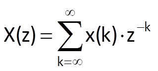
where z is generally a complex variable, usually expressed in the polar form as
or, if we want to retain the physical significance of the exponent, we can write
where r is the modulus of a complex number z and ΩTs (or ΩN, in case of a normalised sampling period) is its argument.
Note
Note that if the variable z is complex, then the function X(z) – which is the result of Z-transform of sequence x(k) – also takes on complex values. It is therefore a complex function of a complex variable.
When working with causal discrete systems, the so-called one-sided (or unilateral) Z-transform can be used. This transform is defined as
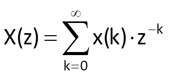
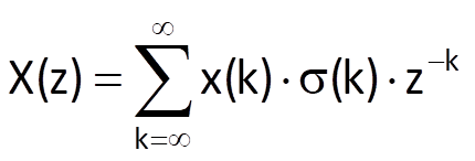
It is obvious that the one-sided and the two-sided Z-transforms have the same characteristics only if x(k) = 0 for k < 0. Formally, a two-sided Z-transform of sequence x(k) multiplied by a discrete unit step can be thought of as a one-sided Z-transform of sequence x(k), i.e.
If we compare the definition of discrete-time Fourier transform (see Eq. 4.1)
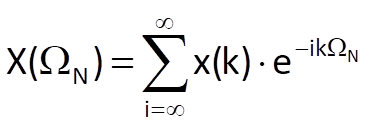 , or better
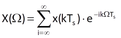
with the definition of Z-transform with substitution z = r.eiΩN (or alternatively, z = r.eiΩTs for r = 1, representing a harmonic kernel function with a unit amplitude), we can see that both equations are equivalent. The discrete-time Fourier transform can therefore be thought of as a specific case of Z-transform.
Example:
Determine the Z-transform of a discrete unit impulse Z(δ(k)), which is defined by
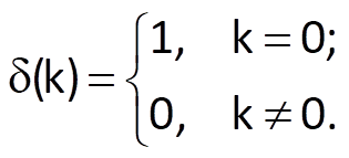
Solution:
We will use the following definition to compute its one-sided Z-transform:
Z(δ(k)) = 1·z0 + 0·z-1 + 0·z-2 + 0·z-3 + … = 1.
Example:
Determine the Z-transform of a time-shifted discrete unit impulse Z(δ(k–i)).
Solution:
For a time-shifted discrete unit impulse it holds
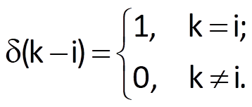
According to the definition, we get the following formula for the one-sided Z-transform:
Z(δ(k-i)) = 0·z0 + 0·z-1 +...+ 0·z-(i-1) +1.z-i + 0·z-(i+1) + … = z-i.
Example:
Determine the Z-transform of a unit-step sequence Z(σ(k)).
Solution:
According to definition of one-sided Z-transform, the Z-transform of a unit step is given by an infinite sum Z(σ(k))= 1 + z-1 + z-2 + z-3 + … . Let us multiply both sides by (z – 1) in order to obtain a more compact expression. We will then get
(z – 1)·Z(σ(k)) = (z – 1)·(1 + z-1 + z-2 +·z-3 + …) = (z + 1 + z-1 + z-2 + …) – (1 + z-1 + z-2 + …) = z.
And finally, we get
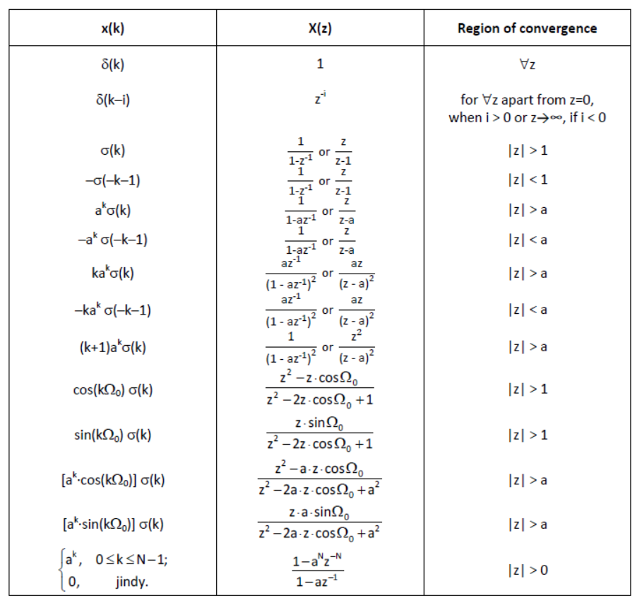
Table 6.1 SEveral common Z-transform pairs
Important characteristics of the Z-transform
- linearity
If sequences x1(k) and x2(k) have Z-transforms X1(z) and X2(z), the following holds:
If R1 and R2 are regions of convergence of Z-transform of sequences x1(k) and x2(k), respectively, then the following holds for the resulting region of convergence R´:
which can be read as: the region R’ is a subset of union of regions R1 and R2.
- time reversion
- time shift of sequence x(k)·σ(k) to the right
- time shift of sequence x(k) to the right
- time shift of sequence x(k) to the left
- multiplication by ak (also called exponential scaling)

in a special case,
- multiplication by k (also called linear scaling)
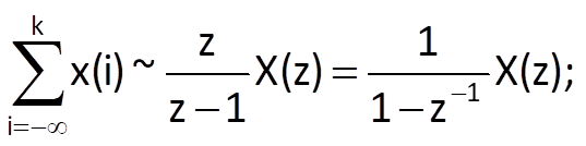
- accumulation
- convolution in the time domain
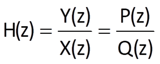
6.3 Transfer function
Now, let us perform the Z-transform of a n-th order difference equation describing a linear system in a general form.
If we write out Eq. (6.2) in the form
then, using Eq. (6.12) and under zero initial conditions, we get
and after a few mathematical operations, we get a formula for the transfer function, which is defined as the ratio of Z-transforms of output and input sequences. Therefore, under zero initial conditions, we get
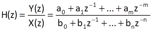
If n ≥ m, we get
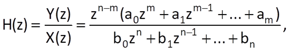
and finally, if m ≥ n, we get
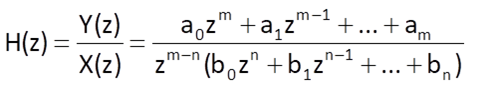
Each of both variants of notations has its advantages. The notation with negative exponents (Eq. (6.21)) indicates a close relation between the transfer function and the difference equation, whereas the variants with positive exponents (Eqs. (6.22) and (6.23) lead to an easier computation of zeros and poles, and therefore to simpler consideration of system stability, as we will see in further chapters. It is certainly also possible to express the transfer function in the form
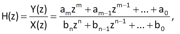
that is just a formal rearrangement, but one should be vary of potentially confusing indices of weighting coefficients ai, bi.
Example:
Determine the transfer function of a system defined by the difference equation
y(k) = 3x(k) – 2x(k – 1) + 2y(k – 1) ‒ y(k – 2).
Solution:
We will move all output-sequence terms to the left side of the difference equation, i.e.
y(k) – 2y(k – 1) + y(k – 2) = 3x(k) – 2x(k – 1)
and then, using Eq. (6.12) and under zero initial conditions, we get
Y(z) – 2z-1Y(z) + z-2Y(z) = 3X(z) – 2z-1X(z)
From this, we easily get the following:
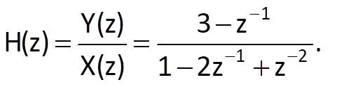
By multiplying both the numerator and the denominator by z2, we get
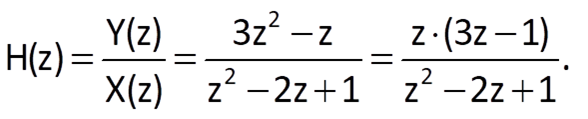
The inverse procedure can be used to determine easily and quickly the system’s difference equation from the transfer function.
Example:
Determine the system’s difference equation from the given transfer function
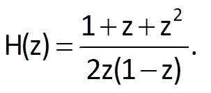
Solution:
Let us multiply both the numerator and the denominator of the given transfer function by z-2. We get
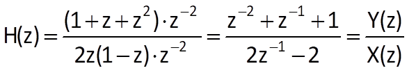
and therefore,
Y(z)(2z-1 – 2) = X(z)(z-2 + z-1 + 1)
Using Eq. (6.12) and under zero initial condition, we get the following difference equation:
2y(k – 1) – 2y(k) = x(k – 2) + x(k – 1) + x(k).
After rearranging this equation into a standard order, we finally get
y(k) = y(k-1) – 0,5x(k) – 0,5x(k-1) – 0,5x(k-2)
Example:
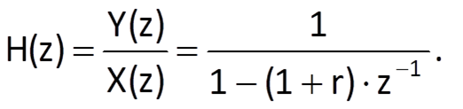
Determine the transfer function from a difference equation describing the behaviour of a nonautonomous linear model of a one-species population.
Solution:
In Chapter 5, we saw a difference equation in the following form, which has only been rewritten using symbols adopted in this chapter:
y(n) = y(n-1).(1+r) + x(n).
A simple rearrangement gives
y(n) - y(n-1).(1+r) = x(n)
and after Z-transform, we get
Y(z) – (1+r) z-1 Y(z). = X(z).
From this, we get the transfer function:
6.4 Distribution of zeros and poles of the transfer function
Apart from the polynomial expression of a transfer function of a linear, time-invariant system, we can express its numerator and denominator by a product of root factors. If we use the form of transfer function according to Eq. (6.24), we get

where am/bn represents a frequency-independent coefficient of system gain and parameters z1, …, zm are roots of the equation
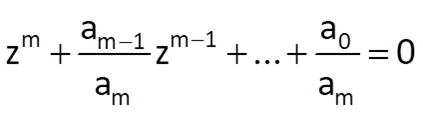
called the zeros of the transfer function and p1, …, pm are roots of the characteristic equation
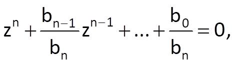
which are called the poles of the transfer function of the system.
6.5 Frequency transfer function and frequency responses
Another possibility of using the transfer function is to determine frequency characteristics of a given system from that function. In other words, to determine how parameters (the amplitude and the initial phase) of a harmonic sequence change after its processing by the system.
If we substitute for the variable z in a transfer function (in the notation according to Eq. (6.24)) according to Eqs. (6.5a) or (6.5b) with the value r = 1, we get a transfer function (for substitution according to Eq. (6.5b)) in the form
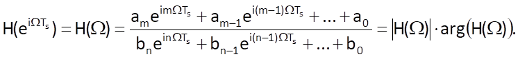
This function is called the frequency transfer function. Because this is again a way of external (input/output) description of linear system characteristics, the function expresses the relation between the input and output sequences of the system or, alternatively, between the harmonic sequences which both sequences are composed of. The magnitude of the frequency transfer function determines the ratio between the amplitudes of harmonic components for a given frequency, which input and output sequences are composed of. Its argument defines the phase (or time) shift between harmonic components of input and output. The dependence of magnitude of values of the frequency transfer function on frequency is called the magnitude frequency response of a discrete system, whereas the dependence of argument of values of the frequency transfer function on frequency is called the phase frequency response.
As we have already mentioned before, the substitution function for the z variable (eq.(6.5), r = 1) is a complex exponential function with a unit modulus, the values of which, in a complex plane, are displayed on a unit circle. For this reason, values of the frequency transfer function are displayed above the unit circle in the complex plane. This fact implies that values of the transfer function repeat periodically, with the argument value equal to integer multiples of 2π. If the argument of the complex exponential function is equal to ΩTs = Ω/fs, then repeating values of this function with an angular period 2π mean that they also repeat with the angular sampling frequency Ωs. In the period <0, Ωs>, values of the frequency transfer function are symmetric about the interval centre, i.e. about the angular frequency Ωs/2. It is obvious that the same applies to the phase frequency response, with the only difference that unlike the magnitude frequency response, the phase frequency response is an odd function, due to the way of its computation.

Figure 6.1 General shape of magnitude of the frequency transfer function.
Example:
Determine the frequency responses of a system described by the difference equation
y(kTs) = x(kTs) + x(kTs – Ts).
Solution:
From the given difference equation, we get the following transfer function:
Y(z) = X(z) + X(z).z-1.
Therefore,
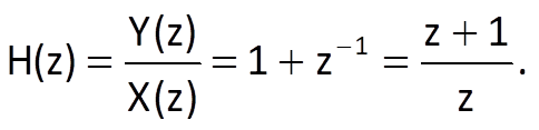
And finally,
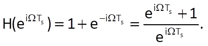
We can obtain a rough estimation of frequency values of ω = 0 and ω = Ωs/2. For ω = 0, 2π, 4π, … the magnitude of the frequency transfer function is equal to
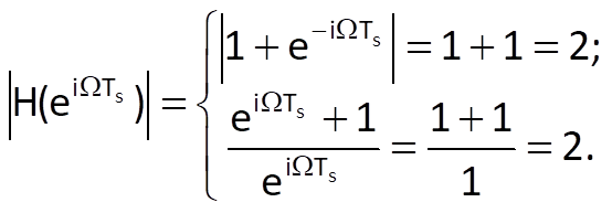
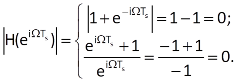
For odd multiples of half of the sampling frequency, the magnitude of the frequency transfer function is equal to
The shape of the magnitude frequency response of the given system is like as it is depicted in Figure 6.2.
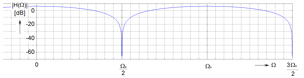
Figure 6.2 Magnitude frequency response of a system given in the example
6.6 Time responses
6.6.1 Impulse response
The definition of transfer function implies that, under zero initial conditions, the following holds for the Z-transform of the output sequence:
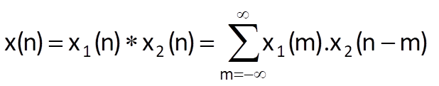
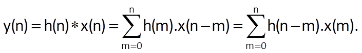
Furthermore, we introduced the concept of convolution in Chapter 2.6.1, expressing the relationship between two sequences of the same argument. According to Eq. (2.33), we get
Subsequently, we saw that the following holds both in the Fourier domain and in the Z-domain (see Eq. (6.18), for example):
or, alternatively,
That means that the Z-transform – or alternatively, the Fourier transform – of a convolution is equal to the product of transforms of both functions entering the convolution.
If Eq. (6.29) says that the Y(z)-transform of output sequence y(n) of a system is given by the product of transfer function of that system with the Z-transform of the input sequence, then it must be possible for us to determine the time course of the output sequence from a convolution of the input sequence with some time series/sequence that would be able to describe the system characteristics. The question is, what time series is that?
Suppose that X(z) = 1 is the transform of input sequence. In that case, we get
This equation implies that the transfer function is equal to the transform of the system’s output sequence, where this transform was produced by a sequence with its Z-transform (or Fourier transform) equal to unity. We know that the unit Dirac impulse is such a function. Consequently, the transfer function of a discrete system is equal to the Z-transform of the system response h(n) to a unit impulse
and vice versa
We can therefore characterise the system by its response h(n) to a unit impulse, which is determined by the inverse Z-transform of the transfer function (or by the inverse Fourier transform of the frequency transfer function). Because this response describes the system characteristics, it is called the system’s impulse response of the system. Unlike all of the so far mentioned ways of description of a linear system, the impulse response has the properties of a time series.
The above-mentioned facts also imply that the system response to any input sequence can be computed as the convolution of time course of the input sequence with the system’s impulse response. Therefore, we get
As demonstrated in Chapter 4.4, a unit impulse has an infinitely wide constant spectrum; that means that applying this sequence to the system input is equal to applying a complete mixture of harmonic sequences with frequencies from 0 to Hz with the same amplitudes. However, no real system is able to transform such a sequence without deformation. We therefore perceive the impulse response as a Dirac impulse deformed by the system, and we can infer the system characteristics based on properties of a sequence deformed in this manner.
In general, the transfer function is given by a rational polynomial function
The system’s impulse response is easiest to compute when Q(z) = 1 or when there is an exact division of polynomials P(z) and Q(z). Then we get
and the impulse response is directly given by values of coefficients ai of the polynomial
Because m < ꝏ , the sequence of coefficients {ai}, i = 0,…,m is also finite and such systems are said to have a finite impulse response (FIR). The opposite case occurs when there is no exact division of polynomials P(z) and Q(z) from the transfer function; such systems are said to have an infinite impulse response (IIR).
Systems with transfer function corresponding to Eq. (6.35) are often called moving average systems (we will use this term in Chapter 7). However, this term evokes a mathematically correct idea that coefficients of the transfer functions are weighted average coefficients, whose sum must be equal to 1. This requirement applied to a domain of systems would mean that a system with such characteristics would have a unit gain, which might not be always necessary and sometimes might not even be desirable. That’s why the systems theory perceives this term – and the requirement following from it – somewhat more broadmindedly.
Example:
Determine the impulse response of a system defined by the following transfer function:

Solution:
We can write the difference equation of a system with the above-mentioned transfer function as:
y(k) - y(k – 1) = x(k) – x(k – 3).
It means that the computation of output sequence also involves the value of output sequence delayed by one sample. This implies a feedback, which might cause certain troubles in computation of the inverse Z-transform. Therefore, let us try out at first whether there is an exact division of both polynomials
(1 – z-3):(1 – z-1) = 1 + z-1 + z-2.
In other words – yes, there is an exact division.
It means we determine the impulse response in the form {1, 1, 1}.
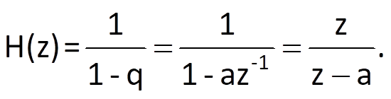
Example:
Determine the transfer function of a system with the impulse response h(k) = ak, a ∈ (0, 1), k ≥ 0.
Solution:
We can write the following for the Z-transform of the given sequence, i.e. for the system’s transfer function:
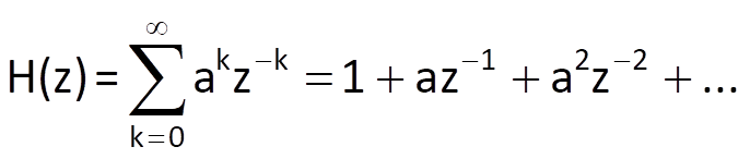
That is an infinite geometric series with quotient az-1 and, given the above-mentioned condition for the value of parameter a, its sum is equal to
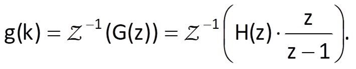
6.6.2 Transient response
Similarly to the impulse response, which is the system’s response to a unit impulse, the system characteristics can also be described by its response to the second fundamental one-shot sequence, i.e. to the unit step. This response is called the system’s transient response and is denoted g(k).
Because the Z-transform of a unit step is (see Table 6.1)

the following holds for the transient response of a system with the transfer function H(z)
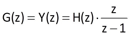
and we get the following formula for its time dependence:
Eq. (6.39) implies that the following is true for transforms of both time responses of a linear system working in discrete time:
According to Eq. (6.17), the expression z.(z – 1)-1 also corresponds to the sum in the time domain, implying that the following holds for both time responses in the time domain:
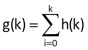
and vice versa
6.7 Mutual relationships between various forms of input/output description of a linear system
Figure 6.3 shows all seven above-mentioned ways of external (input-output) description of linear systems. Connecting lines of various thicknesses are used to illustrate how frequently individual ways of conversions are used: the easier and more frequent is a certain conversion, the thicker is the connecting line between the two corresponding descriptions. In general, it can be stated that all ways of external (input-output) description of linear systems are mutually equivalent (apart from the distribution of zeros and poles); the practicality and difficulty of individual conversions is another question.
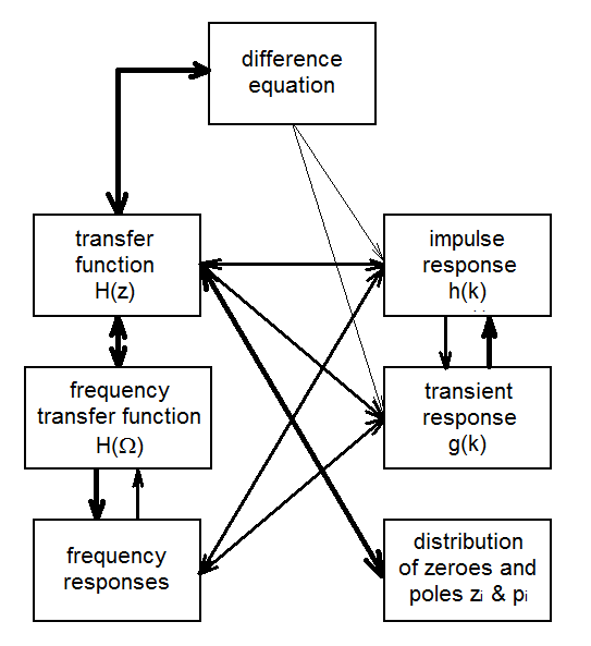
Figure 6.3 Mutual conversion of different forms of external (input-output) description of linear systems.
Many of these conversions were mentioned in chapters dealing with individual forms of description. The conversion between a differential equation and a transfer function, which is based on the Z-transform of delay, is elementary and is used very frequently. The similar is true for the conversion between a transfer function and a frequency transfer function or vice versa or, alternatively, further to frequency responses. The analytical determination of a transfer function (or a frequency transfer function) from measured values of frequency responses is more difficult; in most cases, this is done by an approximation if the system order is supposed or known, or if the requirement on approximation accuracy is given at least. The conversion between time responses is easy, too (the impulse response is a difference between neighbouring samples of the transient response), and the same is true for the conversion between time responses and transfer functions. Relations between the frequency domain and the time domain are not so easy.
Pause for thought:
Why is the distribution of zeros and poles excluded from the exact equivalence of individual ways of the external (input-output) description of linear systems?
6.8 Systems with multiple inputs and outputs
So far, we have only considered systems with one input and one output. How would the situation change if a system had multiple inputs or multiple outputs?
Cases of linear time-invariant systems (i.e. systems with constant parameters) can be solved using the superposition principle. According to this principle, each input can be considered as a separate input while all other inputs are equal to zero. The overall system’s response is then given by the sum of all output responses to separated inputs which, however, were brought to the system at the same time.
Pause for thought:
Is it necessary to solve the case with multiple outputs by using a specific rule or not?