Time Series Jiří Holčík
Biological and many technical systems are complex high-order systems that might often be composed of simpler subsystems. There are three basic ways of connecting systems: serial, parallel and feedback connections. Rules of the so-called block algebra determine the description of other, more complex, systems (for the purposes of their analysis or synthesis, for example). Two basic conditions must be met as prerequisites for the use of block algebra:
- all elements of the system are linear;
- individual block must not influence each other when it is connected to other blocks (i.e. descriptions of individual blocks must remain unchanged after mutual connections of multiple blocks are made).
Many algorithms are based on the block algebra, such as the method of sequential modifications, method of variable elimination, Mason’s rule etc. However, these procedures are somewhat beyond the scope of our reader’s expected knowledge. In the subsequent chapters, we will only deal with the three above-mentioned basic ways of connecting elementary systems.
Chapter 7: Stability, connecting systems
7.1 Stability
7.1.1 Basic terms
Stability can be defined as the system’s capability to keep its behaviour or characteristics within given limits despite potential external disturbances (even despite very turbulent processes going on inside the system). Although this definition is very general, it implies that stability is an internal property of the system. However, it is related to the system’s internal state, which is called the state of equilibrium.
Equilibrium is a relatively stable state of the system that is a result of balance of all the influences having some effect on the system. The equilibrium states can be stable, neutral (also called marginally stable, i.e. on the border of stability) or unstable. In general, stability depends on properties of the system itself (particularly in cases of linear systems) and on the character and influence of the environment on the system (in cases of non-linear systems). We can find out whether the state of equilibrium is stable or unstable by deviating the system a little from its state of equilibrium: if the system returns back to the original state, the system’s original state of equilibrium was stable. If the deviation makes the system leave its original state of equilibrium, then it was unstable. And finally, if a small disturbance deviates the system from its state of equilibrium and the system then remains in the same state that was brought about by the disturbance, then the original state of equilibrium was marginally stable.
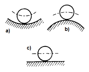
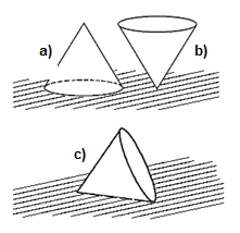
Figure 7.1 Various cases of stable, unstable and marginally stable systems
Figure 7.1 shows examples of these situations. On the left, there is a ball lying on surfaces of different shapes. No matter how the ball is rotated, the ball as such will stay in the same state. The behaviour of the whole system is influenced by the shape of the surface. Situation (a) describes the behaviour of a ball inside a spherical surface of a larger diameter. In this case, no matter how the ball is deviated, it will always return back to the original state of equilibrium, typically by attenuating oscillatory movements: a system in this state of equilibrium is stable. Situation (b) describes the behaviour of a ball on the top of a sphere with a larger diameter. After a deviation from the state of equilibrium, the ball will leave the original position and will not return back – the state of equilibrium is unstable in this case. And finally, situation (c) describes the behaviour of the ball on a flat surface: acted upon by an external force, the ball will move to a new position and will stay in that position; this state of equilibrium is neutral (or marginally stable). On the right, the cone represents a system of which equilibrium states depend on the system itself rather than on properties of the environment in which the system is located. If the cone stands on its base (a), it is in a stable state of equilibrium and a small deviation will not make it overturn. By contrast, if the cone stands on its apex (b), even the smallest deviation will make it tip over. And finally, if the cone lies on its lateral surface (c), it represents a neutral (marginally stable) state of equilibrium: acted upon by an external force, the cone will turn around slightly and will remain in the new position.
To determine the stability of a system, we use two basic approaches that are based on the two following systemic events:
- external stability;
- internal/asymptotic stability (given by convergence of a natural response).
7.1.2 External stability
The external stability is assessed according to the system’s tendency to react adequately to a stimulus of a finite duration and a finite intensity, and according to its tendency to behave after the stimulus has disappeared.
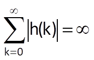
A system is stable if it reacts to each bounded |k(x) (bounded both in terms of intensity and duration) with a bounded output; this is the so-called bounded-input, bounded-output (BIBO) stability. However, only instability can be verified according to this definition: if any input is found after which the system shows an unstable behaviour, the system is unstable. If the system shows a stable behaviour as a reaction to all bounded input sequences that have been tried so far, it does not necessarily mean that there is no input as a result of which the system would show an unstable behaviour.
The so-called Hurwitz’ criterion is a necessary and sufficient condition for this form of stability; in its discrete form, this criterion is written as follows:
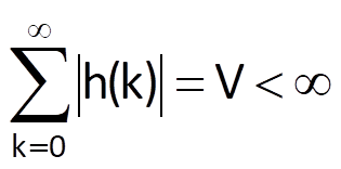
where h(k) is the system’s impulse response. Indeed, if the condition (7.1) is valid and if the input sequence is bounded at the same time, i.e.
we can use the following convolution sum
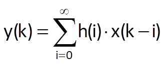
to obtain

The output sequence is bounded and the condition (7.1) is sufficient. Let us prove by contradiction that it is also a necessary condition. Suppose that the Hurwitz condition is not valid, i.e.
yet the system is stable. Let us try and find a sequence which would not meet the basic (abovementioned) condition of BIBO stability, i.e. a sequence which would make the system react to a bounded input with an unbounded output. Let us use the following input sequence:
As a result, we will obtain:

If the Hurwitz condition is not met, the system is unstable. The Hurwitz condition is therefore necessary at the same time.
7.1.3 Internal stability
This type of stability is defined just by properties of the system itself, as its name – internal stability – implies. Internal stability can be therefore recognised from a certain (or in fact, any) description of the system’s properties, as we have mentioned them in the preceding chapter. There are several ways of description of linear systems, and there are also multiple criteria (or methods) to reveal the internal stability in relation to the system’s initial state.
Let us deal with the most common way based on the position of poles of the transfer function; then, let us look at several cases to find the domain in which poles of a stable discrete system must be located.
Formulas shown in Table 6.1 in the preceding chapter imply that if the transfer function – after a partial fraction decomposition – has one root factor with one real pole, the impulse response is h(k) = ak for k ≥ 0. This component sequence converges monotonically if a ∈ (0, 1), k ≥ 0. If the transfer function contains a partial fraction with a pair of complex conjugate poles, the original time series is determined by a formula a.e±iΩ0; in other words, if it contains a root factor with denominator in the form z2 – 2zacosΩ0 + a2, the impulse response contains a sequence of akcos(kΩ0), k ≥ 0. This sequence converges again (not monotonously, but with oscillations) if the modulus of poles is a ∈ (0, 1). These two examples, including possible examples with multiple real root factors, lead to the conclusion that the impulse response of a linear time-invariant system meets the Hurwitz condition of stability if |ai| ∈ (0, 1), i.e. poles of the system’s transfer function are located within the unit circle centred around the origin of a complex plane z. If poles of the transfer function are located on the unit circle, the system is marginally stable.
Example:
Let us consider the non-autonomous linear model of population dynamics of a one-species population which has been derived at the end of Chapter 5, and let us specify conditions for its stability.
Solution:
The derived difference equation had the form y(n) = y(n-1).(1+r) + x(n); the corresponding transfer function, which was determined in Chapter 5, had the form
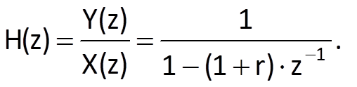
This notation implies that the transfer function has a real pole a = 1 + r. For r > 0 (and therefore, for a > 1, too), i.e. for a positive population increase, the population grows exponentially above all limits and the system is unstable, which corresponds to the description in Chapter 5 and to the abovementioned criterion of stability, too. On the other hand, if r ∈ <-1, 0), the exponential sequence decreases for a negative value of r and the system is stable. Unfortunately, it is the case when the population is dying out.
7.2 Basic ways of connecting systems
Biological and many technical systems are complex high-order systems that might often be composed of simpler subsystems. There are three basic ways of connecting systems: serial, parallel and feedback connections. Rules of the so-called block algebra determine the description of other, more complex, systems (for the purposes of their analysis or synthesis, for example). Two basic conditions must be met as prerequisites for the use of block algebra:
- all elements of the system are linear;
- individual block must not influence each other when it is connected to other blocks (i.e. descriptions of individual blocks must remain unchanged after mutual connections of multiple blocks are made).
Many algorithms are based on the block algebra, such as the method of sequential modifications, method of variable elimination, Mason’s rule etc. However, these procedures are somewhat beyond the scope of our reader’s expected knowledge. In the subsequent chapters, we will only deal with the three above-mentioned basic ways of connecting elementary systems.
7.2.1 Serial connection (cascade connection)
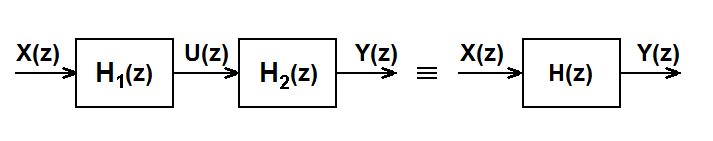
Figure 7.2 Serial connection of two linear systems
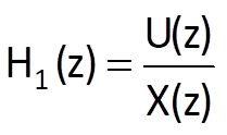
When searching for the relation between transfer functions of two serially connected linear subsystems with transfer functions H1(z) and H2(z) (Fig. 7.2), we proceed from the valid equations
 ;
;
 ,
,
and
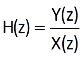 .
.
Further, by expanding the equation for H(z) and by a subsequent simple rearrangement, we obtain

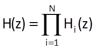
By generalising Eq. (7.10) for a serial connection of N subsystems, we get
In order to derive the equation for the impulse response h(k) of a system given by a serial connection of two subsystems with impulse responses h1(k) and h2(k), we will use the known basic convolution formula describing the relation between the system’s output y(k), its input x(k) and its impulse response h(t)
A serial connection of both subsystems also implies that
Taking into account the validity of associative law for convolution, Eq. (7.13) can be rewritten into the form
or alternatively, if we apply the commutative law:
Comparison of Eqs. (7.12) and (7.15) implies the following formula for a serial connection of two linear systems with impulse responses h1(t) a h2(t)
or alternatively, if we generalise that formula for a serial connection of N systems:
which is a result that might have been expected if we know that the Z-transform of convolution is the product of Z-transforms of original time series and vice versa.
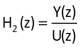
7.2.2 Parallel connection
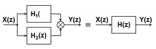
Figure 7.3 Parallel connection of two linear systems
In a parallel connection of two systems (Fig. 7.3), inputs of both systems are identical, whereas their outputs are generally connected by a functional relationship defined in a specific manner. If the resulting system is to be linear as well, outputs must be summed up. Let the transfer functions of the partial systems are defined by the following equations
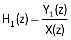
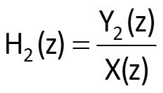
and
Because Y(z) = Y1(z) + Y2(z), we obtain
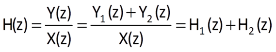
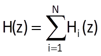
In general, for N systems connected in parallel, we obtain
Now again, let us try to determine the equation for the impulse response of the resulting system. For individual subsystems, we have
and
Because
As with the preceding example, we compare respective equations (7.12) and (7.24); based on this, we get
or alternatively, for a general case of a parallel connection of N systems:
7.2.3 Feedback connection
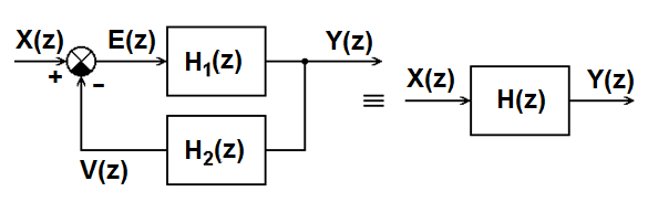
Figure 7.3 Parallel connection of two linear systems
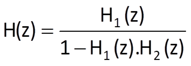
A feedback connection of two systems is shown in Figure 7.4. The system with a transfer function H1(z) is located in the direct branch, whereas the system H2(z) forms the feedback; the output of the feedback system V(z) is either added to or subtracted from the transform of an input sequence X(z) of the whole system, which corresponds to either positive or negative feedback. Let individual transfer functions be defined as
and
Furthermore, if we suppose a negative feedback, we obtain
and therefore
Based on these equations, we can write
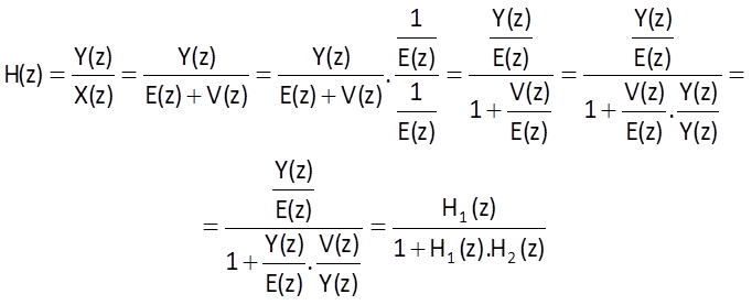
In case of a positive feedback, we obtain
If multiple systems are connected in both branches (either in serial or parallel connection), the transfer function of the entire connection is given by the formula
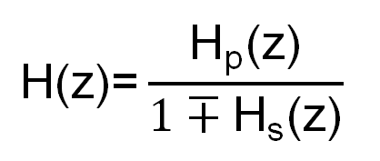
where Hp(z) represents the overall transfer function of the direct branch, whereas Hs(z) represents the product of overall transfer functions of both direct and backward branches of the feedback connection. Determining the impulse response of a feedback connection, based on the knowledge of impulse responses of subsystems, is not as simple as it was in both previously mentioned connections.