Time Series Jiří Holčík
Definition 3.1
Each periodic function x(t+kT) = x(t) which meets the Dirichlet conditions can be decomposed to a Fourier series which, in the exponential form, is given by
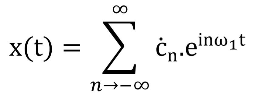
where ċn are complex Fourier coefficients defined by
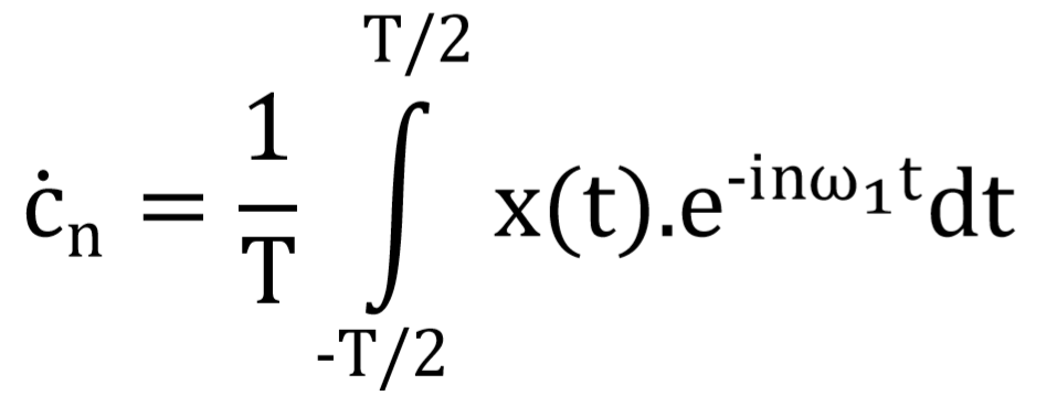
and ω1 = 2π/T is an angular frequency of the first fundamental harmonic component, which is determined by the fundamental period T of the function x(t) to be decomposed.
Module of the complex Fourier coefficient ċn determines the amplitude of the corresponding harmonic component, and its phase determines the value of initial phase of the corresponding harmonic function.
For n = 0, we get
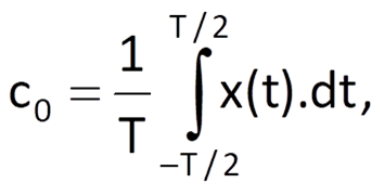
which is the mean value (direct current component) of function x(t).
For real functions x(t), it holds that ċ-n = ċn* (the symbol * is used to mark the complex conjugate value).
Let us take a closer look at Eq. (3.2), which defines coefficients of the Fourier series. Further, remind us of formulas for a mutual correlation of two functions. Then we can see that Eq.(3.2) expresses the correlation function for τ = 0 between the analysed function x(t) and harmonic functions with a zero initial phase and with a frequency equal to integer multiples of angular frequency of the fundamental harmonic component, which is given by period of the function x(t) to be decomposed. In other words, the amplitudes of harmonic components, which the analysed function x(t) is composed of, are given by the level of correlation between the function x(t) and the respective harmonic components. In order to avoid the influence of other harmonic functions (i.e. those with another frequency) on the computation of correlation, it is necessary for the functions controlling the decomposition of the given function – the so-called basis functions (harmonic functions in case of Fourier series) – to be mutually orthogonal over a given interval (period).
Example:
Let us determine parameters of individual harmonic components that make up a train of rectangular impulses (Figure 3.1) with a fundamental period T, duration of individual impulses ϑ and height A. Let the first impulse be placed symmetrically around the origin of time axis.
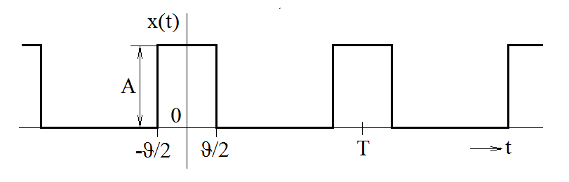
Figure 3.1 Example of a train of rectangular impulses
Solution:
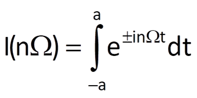
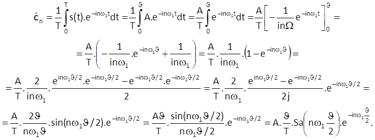
First of all, let us compute the value of an auxiliary integral
For n = 0, we get
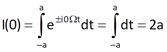
whereas for n ≠ 0, we obtain
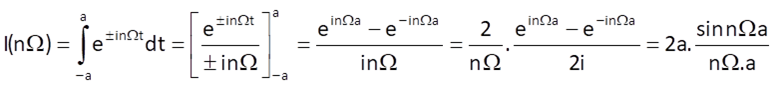
Figure 3.2 shows the shape of the computed function Sa(x) = sin(x)/x. The function is primarily defined by the behaviour of function sin(x), but it is attenuated with a linear growth of x in the denominator. To determine the value of Sa(0) = 1, we will use the limit of the expression sin(x)/x for x → 0, which can be easily computed using the l’Hospital’s rule.
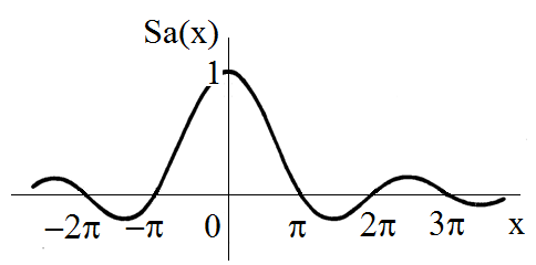
Figure 3.2 Function Sa(x) = sin(x)/x
Based on this result, Fourier coefficients of the above-mentioned train of rectangular impulses can be computed as follows:
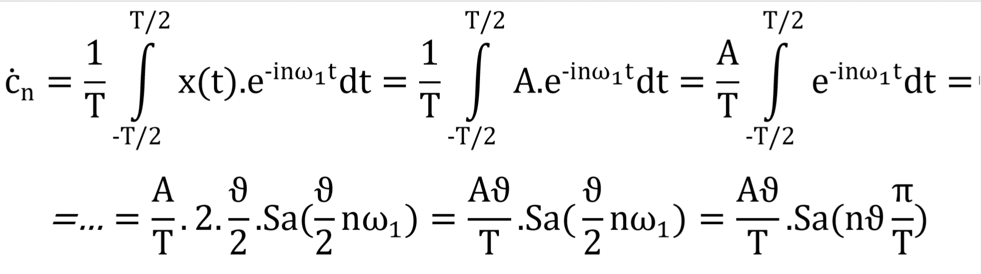
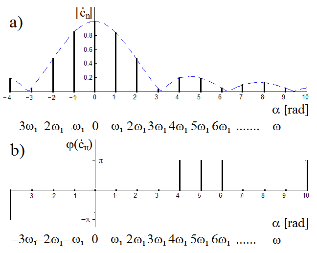
Figure 3.3 (a) Amplitude frequency spectrum (or module frequency spectrum) and (b) phase frequency spectrum of a train of rectangular impulses symmetric around the origin of time axis.
Coefficients ċn take on values of the function Sa(x) for discrete values of the argument ϑnω1/2 multiplied by the expression Aϑ/T, i.e. by the area of one impulse normalised to one period. Because coefficients cn are complex in general, their values can be expressed by dependence of their (a) modules and (b) phases on the frequencies of individual harmonic components; this dependence is called (a) the amplitude frequency spectrum (or module frequency spectrum) and (b) the phase frequency spectrum of a periodic function, respectively. Because our assumptions were based on the exponential form of a Fourier series, both positive and negative values must be expected, and therefore we need to consider frequency components with both positive and negative frequencies.
Graphical representation of values of modules and phases of coefficients ċn for the above-mentioned train of rectangular impulses is shown in Figure 3.3. The periodicity of the analysed function leads to the fact that both parts of the spectrum, i.e. the amplitude frequency spectrum and the phase frequency spectrum, are referred as discrete spectra (or line spectra). This means that the se spectra are only defined for certain frequencies, which are equal to integer multiples of the fundamental harmonic frequency ω1 = 2π/T, where T is the fundamental period of the analysed function. Individual amplitude spectral lines take on values that are just equal to values of the envelope function represented by the dashed line, which is given by the formula
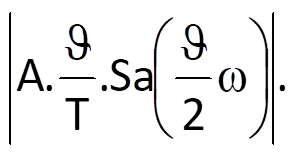
Because the amplitude must be positive, the envelope function is determined by the absolute value. The Sa(x) function is equal to zero for arguments that are integer multiples of π, i.e.
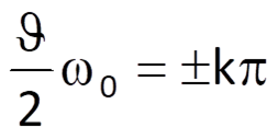
and therefore for the frequency
As follows from Eq. (3.7), the values of Fourier coefficients are purely real and are either positive or negative, depending on the shape of function Sa(x). In a complex plane, this means that the phase of the coefficients is zero only if their values are positive and equal to π (or –π on the negative part of the frequency axis), if values of Fourier coefficients are negative.
Example:
What happens if we shift the train of rectangular impulses from the preceding example in such a way that the rising edge of the rectangle is located at the origin of time axis (Figure 3.4)?
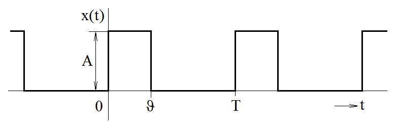
Figure 3.4 Example of a train of shifted rectangular impulses
Solution:
In this case, we will compute the Fourier coefficients as follows:
When we compare the results of both examples, we come to the conclusion that the resulting formulas only differ in the multiplication by an exponential term e-jnω1ϑ/2 (in the second example). What does the multiplication by this term actually mean? Because the complex exponential function eiα represents a complex number with a unit module and a phase α, it means that Fourier coefficients are not purely real numbers in this case; rather, they are generally complex numbers, where the phase α = nω1ϑ/2 is directly proportional to integer multiples of the fundamental angular frequency of the original train of periodic impulses ω1 = 2π/T. If we substitute for ω1 in the power of an exponential term (i.e. nω1ϑ/2), we get α = nπϑ/T. It means that modules of Fourier coefficients stay the same, the only change occurs in their phases, which take on values nπϑ/T for n-multiples of the fundamental harmonic frequency (Figure 3.5).
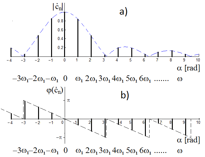
Figure 3.5 (a) Amplitude (or module) frequency spectrum and (b) phase frequency spectrum of the train of rectangular impulses with a rising edge at the origin of the time axis
Chapter 3: Harmonic decomposition of time series. Concept of frequency spectrum. Sampling
3.1 Introduction
As we have already mentioned before, the decomposition of time series to basic components (and, if need be, the subsequent separation of individual components) is the basic analytical activity related to time series processing. The decomposition can be based on a certain a priori knowledge of characteristics of the sought components (often represented by their mathematical models) or just on more or less blind initial assumptions on their properties. A typical assumption of this kind is the assumption that a time series can be additively composed of harmonic sequences with specific characteristics.
At the beginning of the 19th century, Jean B. J. Fourier was historically the first person who described this way of decomposition in his examination of a heat transfer in solid materials. However, this method dealt with the decomposition of variables changing in continuous time. Although characteristics of the resulting harmonic components in this particular case are somewhat different from the results of time series decomposition, they are essential to understand the principles of sampling; that is why we consider it useful to deal with the decomposition of variables in continuous time before anything else. The ways of decomposition of variables in continuous time are principally different, based on their periodicity.
3.2 Decomposition of time-continuous periodic functions to harmonic components
Definition 3.1
Each periodic function x(t+kT) = x(t) which meets the Dirichlet conditions can be decomposed to a Fourier series which, in the exponential form, is given by
where ċn are complex Fourier coefficients defined by
and ω1 = 2π/T is an angular frequency of the first fundamental harmonic component, which is determined by the fundamental period T of the function x(t) to be decomposed.
Module of the complex Fourier coefficient ċn determines the amplitude of the corresponding harmonic component, and its phase determines the value of initial phase of the corresponding harmonic function.
For n = 0, we get
which is the mean value (direct current component) of function x(t).
For real functions x(t), it holds that ċ-n = ċn* (the symbol * is used to mark the complex conjugate value).
Let us take a closer look at Eq. (3.2), which defines coefficients of the Fourier series. Further, remind us of formulas for a mutual correlation of two functions. Then we can see that Eq.(3.2) expresses the correlation function for τ = 0 between the analysed function x(t) and harmonic functions with a zero initial phase and with a frequency equal to integer multiples of angular frequency of the fundamental harmonic component, which is given by period of the function x(t) to be decomposed. In other words, the amplitudes of harmonic components, which the analysed function x(t) is composed of, are given by the level of correlation between the function x(t) and the respective harmonic components. In order to avoid the influence of other harmonic functions (i.e. those with another frequency) on the computation of correlation, it is necessary for the functions controlling the decomposition of the given function – the so-called basis functions (harmonic functions in case of Fourier series) – to be mutually orthogonal over a given interval (period).
Example:
Let us determine parameters of individual harmonic components that make up a train of rectangular impulses (Figure 3.1) with a fundamental period T, duration of individual impulses ϑ and height A. Let the first impulse be placed symmetrically around the origin of time axis.
Figure 3.1 Example of a train of rectangular impulses
Solution:
First of all, let us compute the value of an auxiliary integral
For n = 0, we get
whereas for n ≠ 0, we obtain
Figure 3.2 shows the shape of the computed function Sa(x) = sin(x)/x. The function is primarily defined by the behaviour of function sin(x), but it is attenuated with a linear growth of x in the denominator. To determine the value of Sa(0) = 1, we will use the limit of the expression sin(x)/x for x → 0, which can be easily computed using the l’Hospital’s rule.
Figure 3.2 Function Sa(x) = sin(x)/x
Based on this result, Fourier coefficients of the above-mentioned train of rectangular impulses can be computed as follows:
Figure 3.3 (a) Amplitude frequency spectrum (or module frequency spectrum) and (b) phase frequency spectrum of a train of rectangular impulses symmetric around the origin of time axis.
Coefficients ċn take on values of the function Sa(x) for discrete values of the argument ϑnω1/2 multiplied by the expression Aϑ/T, i.e. by the area of one impulse normalised to one period. Because coefficients cn are complex in general, their values can be expressed by dependence of their (a) modules and (b) phases on the frequencies of individual harmonic components; this dependence is called (a) the amplitude frequency spectrum (or module frequency spectrum) and (b) the phase frequency spectrum of a periodic function, respectively. Because our assumptions were based on the exponential form of a Fourier series, both positive and negative values must be expected, and therefore we need to consider frequency components with both positive and negative frequencies.
Graphical representation of values of modules and phases of coefficients ċn for the above-mentioned train of rectangular impulses is shown in Figure 3.3. The periodicity of the analysed function leads to the fact that both parts of the spectrum, i.e. the amplitude frequency spectrum and the phase frequency spectrum, are referred as discrete spectra (or line spectra). This means that the se spectra are only defined for certain frequencies, which are equal to integer multiples of the fundamental harmonic frequency ω1 = 2π/T, where T is the fundamental period of the analysed function. Individual amplitude spectral lines take on values that are just equal to values of the envelope function represented by the dashed line, which is given by the formula
Because the amplitude must be positive, the envelope function is determined by the absolute value. The Sa(x) function is equal to zero for arguments that are integer multiples of π, i.e.
and therefore for the frequency
As follows from Eq. (3.7), the values of Fourier coefficients are purely real and are either positive or negative, depending on the shape of function Sa(x). In a complex plane, this means that the phase of the coefficients is zero only if their values are positive and equal to π (or –π on the negative part of the frequency axis), if values of Fourier coefficients are negative.
Example:
What happens if we shift the train of rectangular impulses from the preceding example in such a way that the rising edge of the rectangle is located at the origin of time axis (Figure 3.4)?
Figure 3.4 Example of a train of shifted rectangular impulses
Solution:
In this case, we will compute the Fourier coefficients as follows:
When we compare the results of both examples, we come to the conclusion that the resulting formulas only differ in the multiplication by an exponential term e-jnω1ϑ/2 (in the second example). What does the multiplication by this term actually mean? Because the complex exponential function eiα represents a complex number with a unit module and a phase α, it means that Fourier coefficients are not purely real numbers in this case; rather, they are generally complex numbers, where the phase α = nω1ϑ/2 is directly proportional to integer multiples of the fundamental angular frequency of the original train of periodic impulses ω1 = 2π/T. If we substitute for ω1 in the power of an exponential term (i.e. nω1ϑ/2), we get α = nπϑ/T. It means that modules of Fourier coefficients stay the same, the only change occurs in their phases, which take on values nπϑ/T for n-multiples of the fundamental harmonic frequency (Figure 3.5).
Figure 3.5 (a) Amplitude (or module) frequency spectrum and (b) phase frequency spectrum of the train of rectangular impulses with a rising edge at the origin of the time axis
3.3 Decomposition of time-continuous non-periodic functions to harmonic components
3.3.1 Fourier transform
As we have mentioned before, non-periodic functions can be considered periodic with an infinitely long period. Frequency of the fundamental harmonic component of a periodic function is
and therefore, we can write for T→ ꝏ :
This represents getting spectral lines closer when periods prolong. In the limit case when T→ꝏ the distance between spectral lines approaches zero. Therefore, In a non-periodic function, the spectral lines will form a continuous spectrum, the discrete representation of angular frequencies of individual harmonic components will become a continuous variable, and the equation defining the Fourier series (e.g. Eq.(3.1)) will change from its summation form to an integrative form, where coefficients ċn will be determined on the basis of the following considerations.
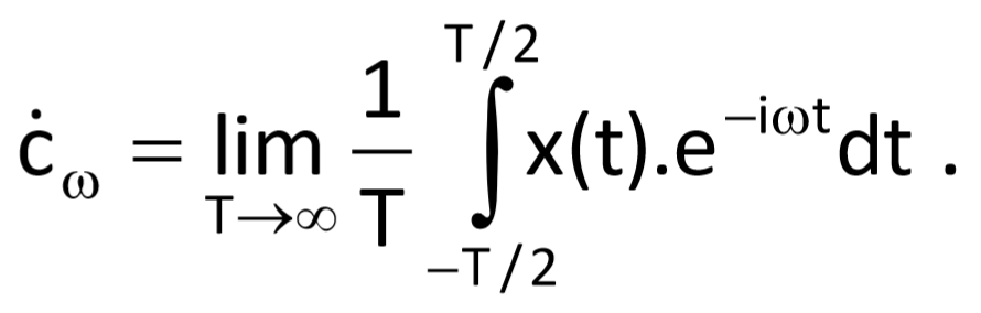
In Eq. (3.2), i.e.
we have T = 2π/dω and therefore, we get T → ꝏ a nω1 → ω for the limit difference of two neighbouring frequencies (dω → 0). Further, for a non-periodic function (in other words for the periodic function with an infinite period), the integral limits will be –ꝏ and +ꝏ. Amplitudes of the continuous spectrum of a non-periodic function will be infinitely small for T → ꝏ, as well. If we express the Eq. (3.2) in a limit form, we get
The definition of Fourier decomposition is then transformed to the form
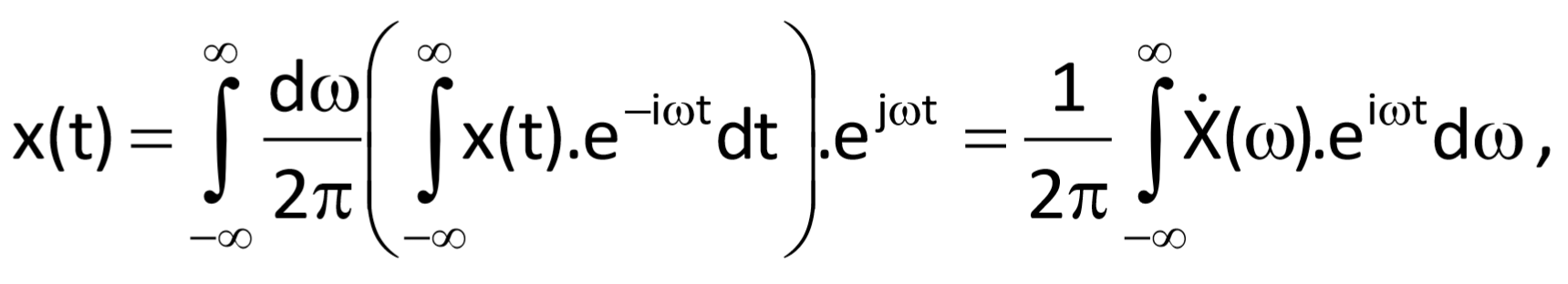
where the equation
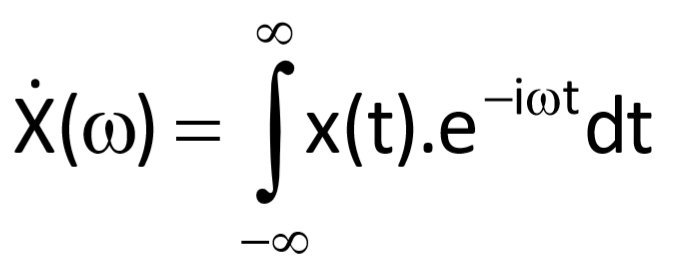
represents the Fourier transform. Resulting function Ẋ(ω) is referred to as the spectral function or spectral density of the function x(t),. The linear integral Fourier transform converts the function x(t) from the time domain to a function Ẋ(ω) in a frequency domain. In order that the Fourier transform may be computable, it is sufficient when the function x(t) is absolutely integrable on the interval (–ꝏ, ꝏ). The spectral function does not express actual amplitudes of harmonic components which the transformed function consists of (as it was the case of the decomposition by the Fourier series); but it describes their proportional relationships only.
Eq. (3.12) defines an inverse relationship, i.e. the way of computation of time representation of a variable from its spectral function. It is called the inverse Fourier transform.
3.3.2 Properties of the Fourier transform
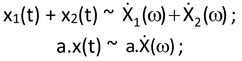
Without derivations and without more detailed explanatory comments, let us mention the following basic characteristics of Fourier transform (we use the notation x(t) ~ Ẋ(ω) to express that Ẋ(ω) is a spectral function of the function x(t)):
- linearity – superposition principle
- time reversal
- time scaling
- time shifting
- frequency shifting
3.3.3 Handful of examples to illustrate the spectral function
Example:
Let us determine the spectral function of a unit step
Solution:
A unit step σ(t) is defined as follows, for example
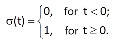
Unfortunately we can see from Eq.(3.19), that the unit step does not meet the condition of absolute integrability, i.e. the Fourier integral does not exist. Therefore, we will use the exponential function to help us:
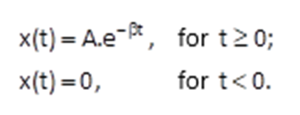
Because the function has a non-zero value only for t ≥ 0, the Fourier integral can only be used in the interval from 0 to ꝏ . That is why we obtain
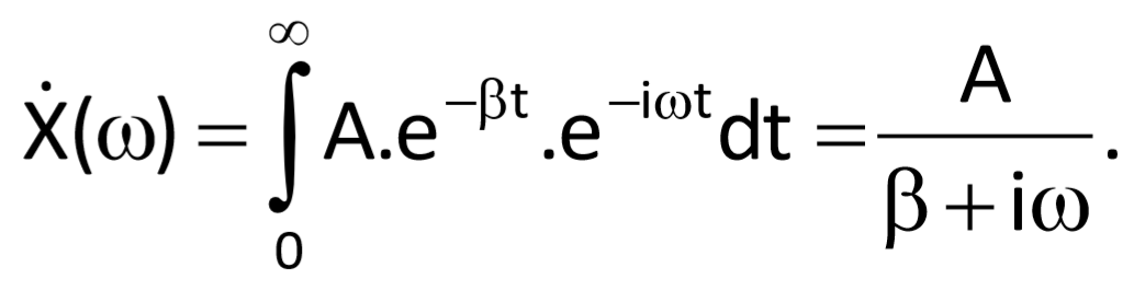
The above-mentioned exponential function can be thought of as a unit step provided that attenuation ß = 0 and coefficient A = 1. Then
and therefore
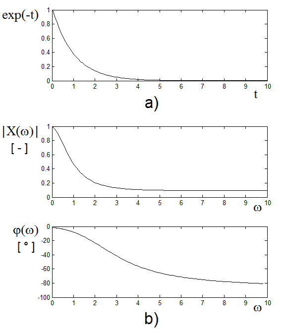
Figure 3.6 Graph of e-ßt, ß = 1 and its spectral representation
Figure 3.7 Graph of the unit step function and its spectral representation
Example:
Determine the spectral function of a rectangular impulse with height A, duration t and rising edge at the origin of the time axis.
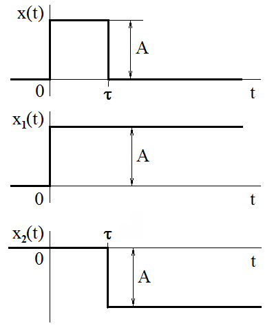
Figure 3.8 Construction of a rectangular impulse from mutually shifted step functions
Solution:
A rectangular impulse with the required characteristics can be constructed from mutually shifted step functions, as it is shown in Figure 3.8. We computed the spectrum of a unit step in the preceding example, and the influence of a time shift on the spectrum is described in Chapter 3.3.2. Therefore, the following holds:
Then we get
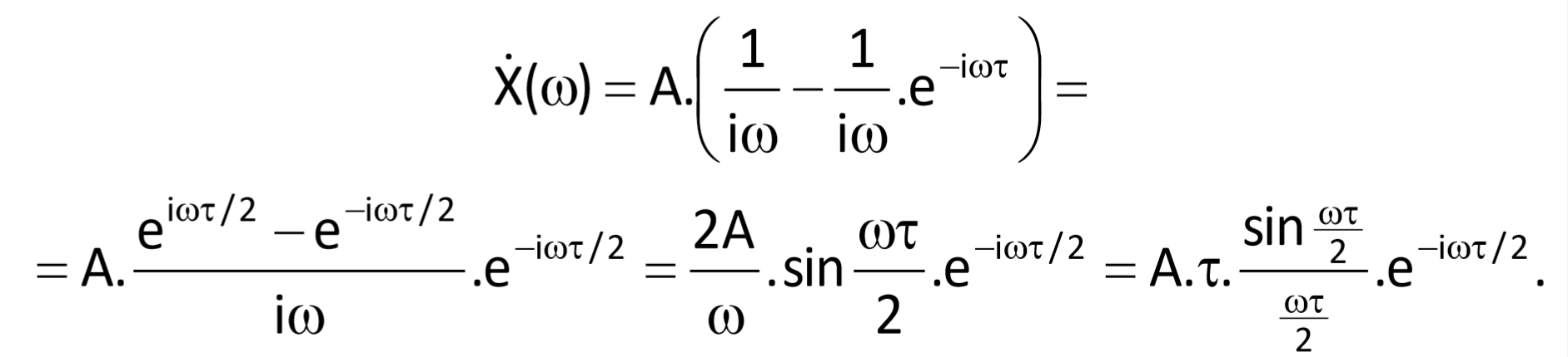
This implies that the module of the spectral density is given by τπ
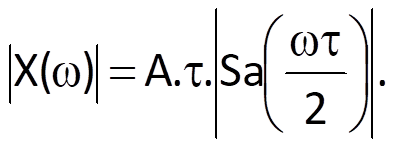
The module of spectral function is given by the function Sa(ωτ/2). This function is equal to zero for arguments equal to integer multiples of π, i.e. for
or alternatively
and therefore
This means the narrower the rectangular impulse is, the flatter its modular spectral function is.
The phase spectrum is given by sum of the function
and the phase following from a change of the sign of the function Sa(ωτ/2).
Example:
Determine the spectrum of a Dirac unit impulse.
Solution:
So far, we have only introduced a discrete unit impulse; therefore, it is necessary to define a Dirac impulse in a continuous time domain.
Informally, it is a function δ(t) which equal to zero at all values of the real axis apart from zero, where it tends to infinity, i.e.
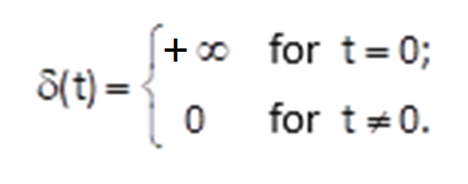
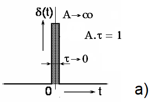
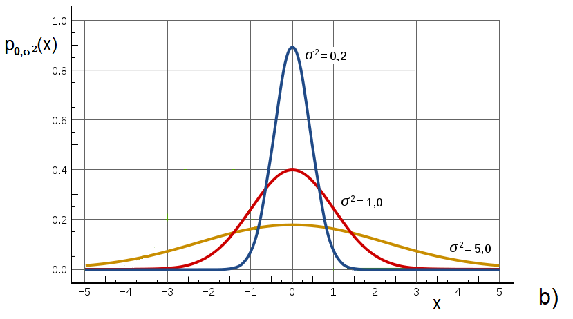
Figure 3.9 Various mathematical expressions of a unit impulse
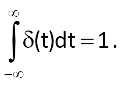
It must be valid for the Dirac impulse that
For simplicity’s sake, we can say that a unit impulse δ(t) is an infinitely narrow and infinitely high rectangular impulse, whose height is equal to the reciprocal of width, i.e. the area delineated by the impulse and the time axis is equal to one (Figure 3.9, left).
Characteristics of the Dirac impulse can be also clearly understood from the limit relationship for a normal distribution with the zero mean and the variance s approaching zero (Figure 3.9, right).
With Eq. (3.32) in mind, we also have
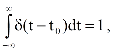
where the argument of the delta function represents shifting the impulse by the value t0 in the positive direction along the time axis. Based on this equation, the following can be derived:
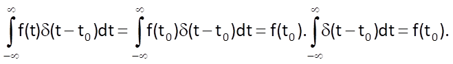
The geometric interpretation of this result can be that the area delimited by the product of a continuous function f(t) and a unit impulse δ(t – t0) is equal to the value of function f(t0) in the moment where the unit impulse occurs. This property is called the sampling property of a unit impulse (Figure 3.10).
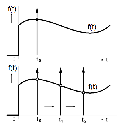
Figure 3.10 Sampling property of a unit impulse
We can see that the Dirac impulse has somewhat anomalous characteristics. Therefore, let us try and solve the problem preferably by a simple reasoning based on previously achieved results.
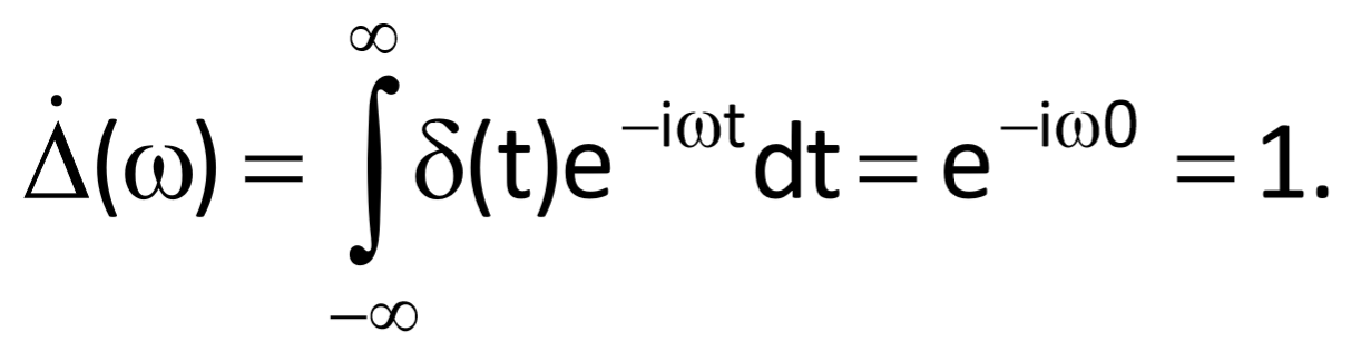
Because a unit impulse can be thought of as an infinitely narrow and infinitely high rectangular impulse (where the product of width and height is equal to 1), the product A.τ defining the multiplication coefficient in a modular spectral function of the rectangular impulse (Eq (3.25)) is equal to unity, and the spectral function is equal to zero for the first time when ω → ꝏ. This means that the module of spectral function of a unit impulse is equal to 1 for all frequencies and that the phase is zero in the entire range of frequencies.
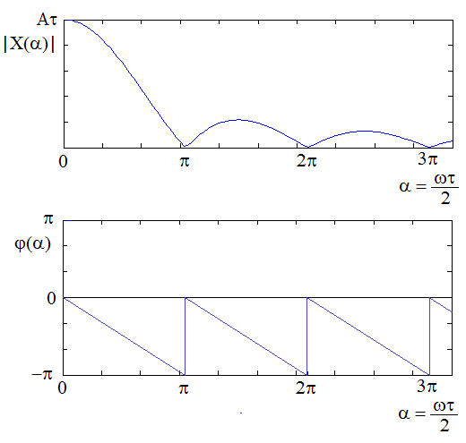
Figure 3.11 Spectral function of a rectangular impulse: (a) module spectrum; (b) phase spectrum
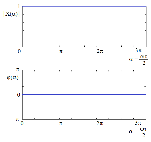
Figure 3.12 Spectral function of a unit impulse
Based on (3.13) and (3.35), we can also write
Example:
Determine the spectrum of a periodic sequence of Dirac impulses with a period T.
Solution:
Similarly to the case of a one-shot unit impulse, this problem can be solved using the analysis of the previously solved example of a periodic train of rectangular impulses.
Periodic character of the signal implies that its spectrum must be discrete and that it takes on values only for frequencies equal to integer multiples of the fundamental angular frequency, which is given by the period T of the pulses, i.e. nΩ = 2πn/T. Because the values of modules of Fourier coefficients ċn determined for a rectangular impulse are given by values of the function Sa(ϑω/2) (see Figure 3.3) and because the duration of individual impulses ϑ approaches zero, position of the first zero value of the function Sa(ϑω/2) approaches infinity. Therefore, modules of individual coefficients take on constant values equal to |ċn| = 1/T and, due to positive real values of these coefficients, the phase is equal to zero.
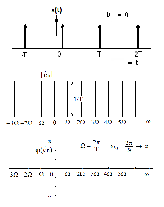
Figure 3.13 Periodic sequence of unit impulses and its spectral functions
Example:
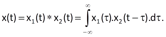
Suppose that a function x1(t) has a spectral function Ẋ1(ω) and that a function x2(t) has a spectral function Ẋ2(ω). Determine the relation for a Fourier transform of the function equal to a convolution of both component functions x1(t) and x2(t).
Solution:
Convolution x(t) of two component functions x1(t) a x2(t) is given by
The Fourier transform of a function x(t) is determined as follows:
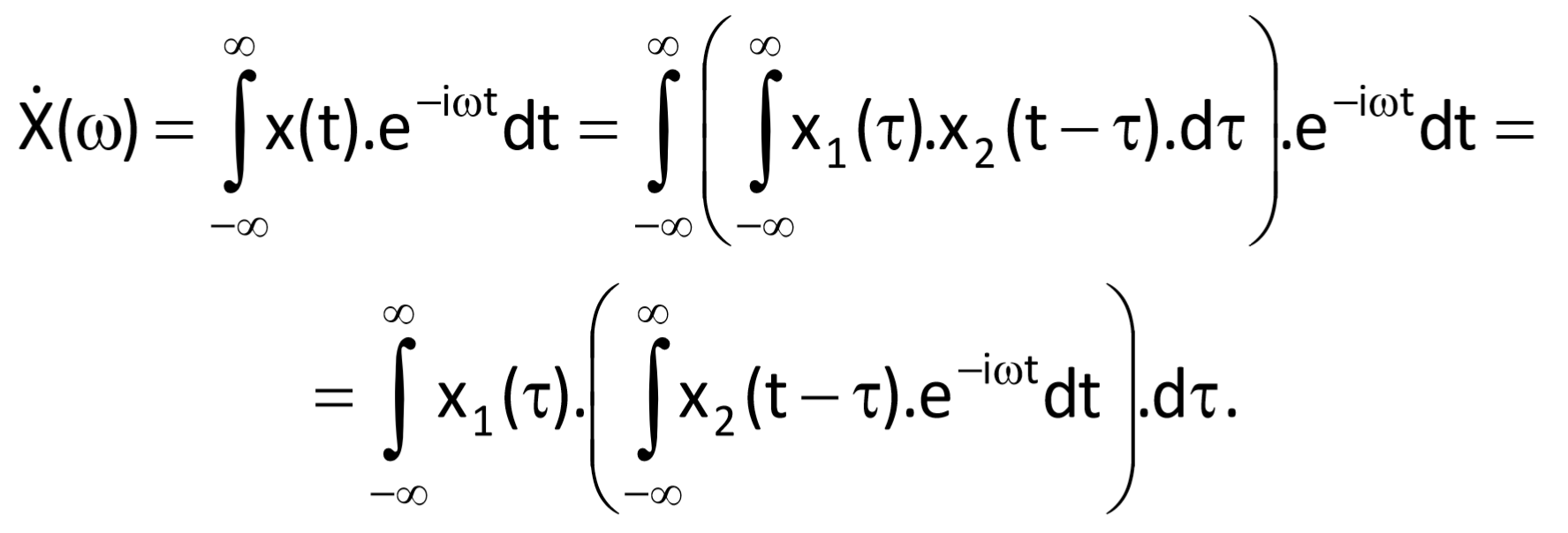
The inner integral represents the Fourier transform of function x2(t) shifted by τ in time. According to Eq. (3.17), it holds for the spectrum of such a function:
If we substitute from this relationship to Eq. (3.17), we get
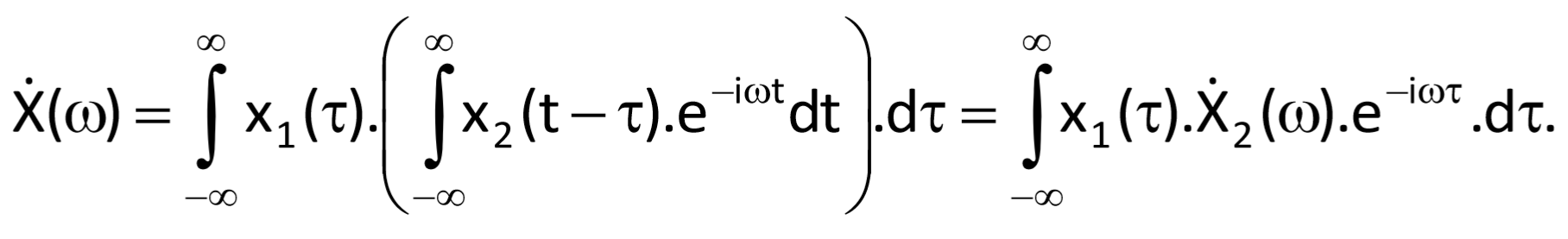
Because Ẋ2(ω) is not a function of τ, we can factor out this term from the integral
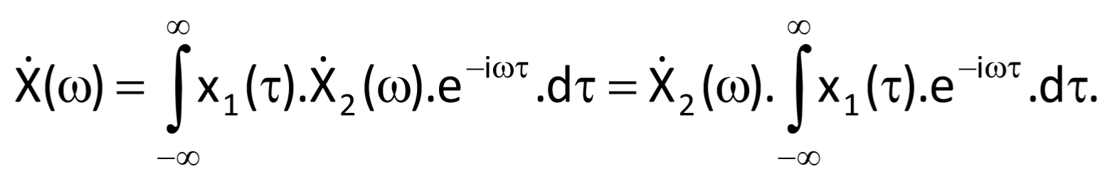
In this case, integral in the second part of Eq. (3.38) represents the Fourier transform of function x1(τ) – or alternatively, x1(t); therefore, it is
3.4 Sampling of time-continuous variables – sampling theorem
The term “sampling” refers to the process of selecting values at specific moments from a variable defined in a continuous time domain. In general, these moments can be distributed along time axis either regularly or irregularly. However, from a point of view of data processing, an regular distribution of sample positions is more convenient.
In case that time is the independent variable, the principle of sampling any continuous variable is shown in Figure 3.14; the distances between individual samples are equal to time periods Ts: this is called the sampling period.
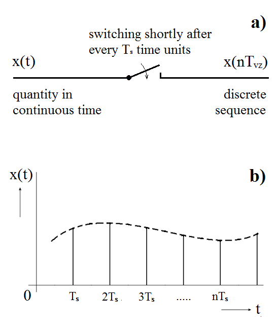
Figure 3.14 (a) The principle of sampling; (b) a continuous function and its sampled variant
In order to simplify the analysis of sampling influence on the characteristics of the sampled variable, the sampled version of the originally continuous variable x(t) is expressed in the form x(t).p(t), where p(t) is the periodic sequence of unit impulses, defined as
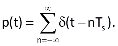
Therefore, the following relation holds for the sampled variable:
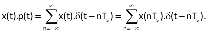
This relation implies that the sampled variable x(t).p(t) is given by a sequence of impulses levels of which are equal to values of samples of the original variable at time points nTs. (Sampling described by Eq. (3.41) is referred to as an ideal sampling.)
Determining the duration of sampling period Ts or, alternatively, sampling frequency fs = 1/Ts or ωs = 2π/Ts, is an important step in the sampling process.
The minimum value of the sampling frequency, which is given by the reciprocal of the sampling period, is determined by the so-called sampling theorem, which is often associated with Claude E. Shannon, Harry T. Nyquist or Vladimir A. Kotelnikov. This theorem says that an exact reconstruction of a continuous, frequency-restricted variable from its samples would be theoretically feasible if this variable was sampled with a frequency fs at least two times higher than the maximum frequency of the reconstructed variable. Mathematically expressed, it must hold:
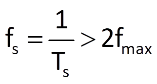
where fmax is frequency of the harmonic component with the highest frequency from all harmonic components involved in a given variable. In case of irregular sampling, Eq. (3.42) must hold for the mean value of sampling frequency.
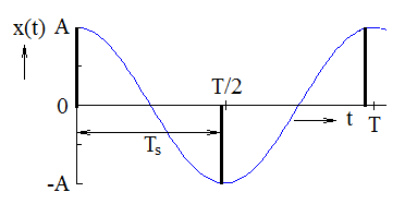
Figure 3.15 The principle of explanation of the sampling theorem
The above-mentioned statement can be derived mathematically, of course. But first, let us content ourselves with the following relatively simple reasoning. As we have mentioned before, a harmonic function is given by three parameters: the amplitude, the frequency and the initial phase. In order to be able to determine these three parameters, we need three equations for three independent values of the function in three different moments in a single period (because a harmonic function is periodic). When the distances between individual time points are to be equal, it is necessary that the time period between them (i.e., the sampling period) is shorter than half of the period of the harmonic function (Figure 3.15). If we want this rule to hold for the harmonic component with the highest frequency, the sampling period must be shorter than half of the period of this harmonic component.
A somewhat more sophisticated explanation of the sampling theorem is based on spectral properties of a sampled continuous function.
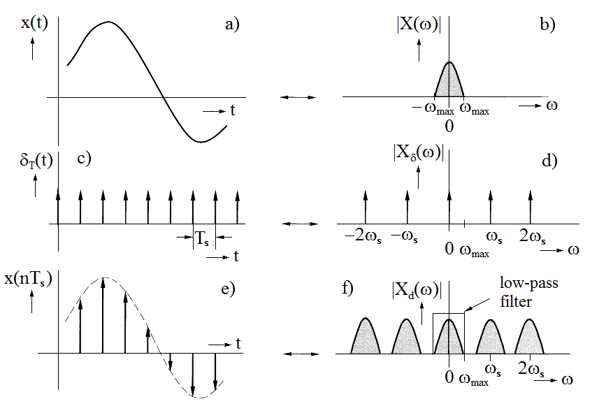
Figure 3.16 Signal sampling and its spectrum
Let the sampled function x(t) (Figure 3.16a) have a spectrum shown in Figure 3.16b. The train of Dirac impulses with a period Ts has a spectrum in the form of a periodic sequence of Dirac impulses in a frequency domain with a period ws, as determined in the example at the end of Chapter 3.3.3 and as shown in Figure 3.16d. Because the sampled sequence is given by a product of the original continuous function and the train of unit impulses (see Eq. (3.41)), the resulting spectrum of the sampled sequence is given by a convolution of both the component spectra. And because one of the defining characteristics of a unit impulse says that the result of its convolution with a given function is the value of function at the point of occurrence of the unit impulse, the resulting spectrum has the form as it is shown in Figure 3.16f. It has a periodic character with a period equal to the sampling frequency, and shapes of individual segments correspond to the shape of spectrum of the sampled function. Therefore, sampling of a time-continuous function makes frequency spectrum periodic, with individual spectral periods having the shape of spectrum of the original sampled signal. The figure demonstrates that individual segments of the spectrum will not overlap provided that the maximum frequency of signal components is not higher than half of the sampling frequency.
Figure 3.16 – and Figure 3.17, in particular – show how it is possible to convert a discrete sequence back to a continuous function. This can be achieved by suppressing those parts of the spectrum which are located around non-zero multiples of the sampling frequency. This suppression is performed by a selective system that can let pass through harmonic components of a sequence with lower frequencies and suppresses components with higher frequencies; such an algorithm (filter) is called a low-pass filter. If the sampling frequency just satisfied the sampling theorem (fs = fmax), the resulting spectrum would have the shape as shown in the upper part of Figure 3.17. In terms of the backward conversion, this would mean that the used low-pass filter should have ideal shape, i.e. it should retain harmonic components of a discrete sequence with frequencies up to fs/2 without any distortion and, by contrast, it should completely remove all harmonic components with frequencies higher than fs/2. Unfortunately, such an ideal system is impossible to construct in real life. That is why, when solving real problems, it is necessary to use sampling leading to a somewhat less distinctive situation, i.e. to use a sampling frequency higher than that exactly defined by the sampling theorem.
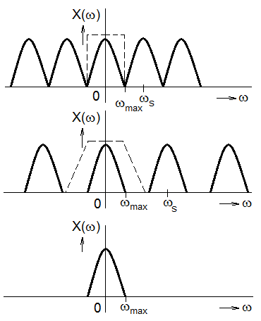
Figure 3.17 The spectral principle of a backward conversion of a discrete sequence to a continuous variable
In practice, the sampling frequency is typically chosen to be two times higher than the maximum frequency contained in the signal, plus a certain reserve. For example, in telecommunications, the frequency of 8 kHz is used to transfer telecommunication signals in the standard frequency band ranging from 0.3 to 3.4 kHz. When recording sound to a CD, the sampling frequency is 44.1 kHz, because a healthy human ear can hear sounds with a maximal frequency of 20 kHz. In medical signals, the reserve is generally higher: the sampling frequency is nowadays chosen to be up to four or five times higher than the maximum frequency in the spectrum.
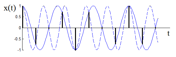
Figure 3.18 The aliasing principle – if a signal with a higher frequency (dashed curve) is undersampled with a frequency lower than the one implied by the sampling theorema, the reconstructed signal (solid line) has a frequency following from the assumption that the sampling theorema was respected.
If the sampling theorem was not met – i.e. if the sampling frequency was lower than twice the maximum frequency contained in the signal (i.e. the signal would be undersampled), the phenomenon called aliasing (or spectral overlapping) would occur. The impact of undersampling can be seen both in the time domain and in the frequency domain. In the time domain, the reconstructed function would have lower frequencies when compared to the original sampled function (Figure 3.18). Displaying the effects of undersampling in the frequency domain demonstrates why the phenomenon is referred to as spectral overlapping (Figure 3.19). The so-called stroboscopic effect is also related to the demand on the sampling frequency. Due to this effect, wheels on a horse-drawn wagon appear to be turning backwards when there is a certain ratio of wheel-turning frequency and the frequency of film shots. Application of the low sampling frequency and the fact that the spectrum of a discrete sequence is periodic lead to a phenomenon when the maximum frequency of a discretised (i.e. sampled) function exceeds the half of sampling frequency and both parts of the spectrum add up. The more pronounced undersampling is, the more smoothed is the resulting spectrum (for a given shape of the spectral function).
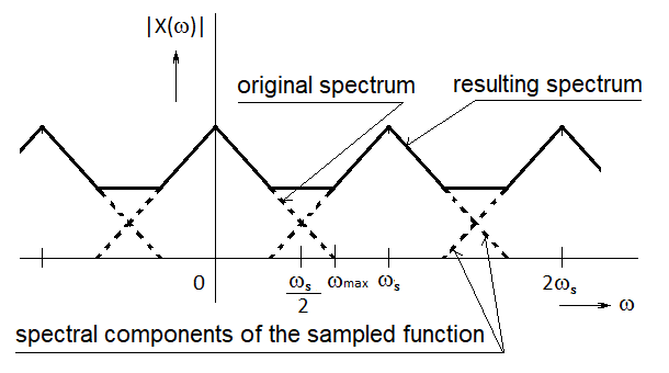
Figure 3.19 Spectral overlap ue to an unsuitable sampling frequency