Time Series Jiří Holčík
Experiments and observations in experimental disciplines such as physics, chemistry, biology, medicine, sociology, economics or technical disciplines – but also psychology, musicology or criminalistics – generate data varying in time, which somehow describe dynamic properties and function of the data-generating subject. The variables of which values are measured are usually defined at any time; such variables are said to be continuous in time (Figure 1.1.). However, values of monitored variables are rarely measured continuously in time: either it is not possible at all or it actually might be possible but we do not want to perform continuous measurement for various reasons (for example, it would be too expensive or too difficult to implement in terms of organisation or technology; furthermore, the way of subsequent data processing must also be taken into account). We typically only determine some of their values – the so-called samples. We therefore obtain a sequence of discrete-time values (Figure 1.1), which is called a time series.
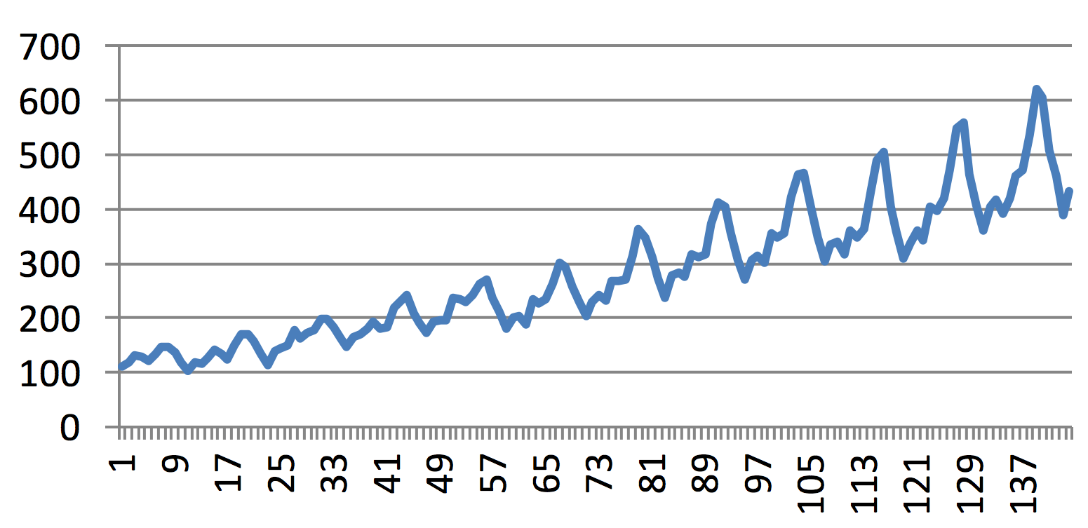
Figure 1.1 One of the classic time series – monthly numbers of passengers travelling with one of American airline in the period from January 1949 to December 1960.
Definition 1.1
A time series is a time-ordered set of values {y(ti): i = 1,…,N}, where ti determines the time at which value y(ti) was determined.
In cases where points in time (ti) are distributed regularly on the time axis, the above-mentioned notation is usually simplified to the form {yt: t = 1,2,…n}. However, this way of notation suppresses the dependence of monitored variable(s) on time, replacing it by a mere dependence on order, which can be undesirable in various situations. On the other hand, this notation makes it possible to use the theoretical apparatus of time series for other forms of dependence (for example, dependence on spatial coordinates).
Properties and the way of further processing of a time series depend on the character of values of the above-mentioned parameters – number of samples or simultaneously recorded variables, sampling rate, character of values, and on several more factors.
Chapter 1: Introduction & Motivation
1.1 Introduction
Experiments and observations in experimental disciplines such as physics, chemistry, biology, medicine, sociology, economics or technical disciplines – but also psychology, musicology or criminalistics – generate data varying in time, which somehow describe dynamic properties and function of the data-generating subject. The variables of which values are measured are usually defined at any time; such variables are said to be continuous in time (Figure 1.1.). However, values of monitored variables are rarely measured continuously in time: either it is not possible at all or it actually might be possible but we do not want to perform continuous measurement for various reasons (for example, it would be too expensive or too difficult to implement in terms of organisation or technology; furthermore, the way of subsequent data processing must also be taken into account). We typically only determine some of their values – the so-called samples. We therefore obtain a sequence of discrete-time values (Figure 1.1), which is called a time series.

Figure 1.1 One of the classic time series – monthly numbers of passengers travelling with one of American airline in the period from January 1949 to December 1960.
Definition 1.1
A time series is a time-ordered set of values {y(ti): i = 1,…,N}, where ti determines the time at which value y(ti) was determined.
In cases where points in time (ti) are distributed regularly on the time axis, the above-mentioned notation is usually simplified to the form {yt: t = 1,2,…n}. However, this way of notation suppresses the dependence of monitored variable(s) on time, replacing it by a mere dependence on order, which can be undesirable in various situations. On the other hand, this notation makes it possible to use the theoretical apparatus of time series for other forms of dependence (for example, dependence on spatial coordinates).
Properties and the way of further processing of a time series depend on the character of values of the above-mentioned parameters – number of samples or simultaneously recorded variables, sampling rate, character of values, and on several more factors.
1.1.1 Main idea
In principle, any time series consists of two basic components. The first component is deterministically related to properties of the monitored subject; these properties are the subjects of research. If this component was not present in values of a given time series, there would be no reason at all to process that time series.
Examples:
The patient’s raised temperature and its development in time is related to response of the pa-tient’s immune system.
The evoked component in electroencephalographic signal is a reaction to a sensory (acoustic, visual, mechanic, …) stimulus.
The exchange rate of a currency is related to statements by the national bank representatives.
The development of a political party preference is determined, among others, by media cam-paigns, both positive and negative.
The second component represents everything that is not the subject of research. This can be data related to the activity of a given subject, which are however not important with respect to the purpose of research; it can also be parasitic disturbance, which got into the time series either from the environment or during the process of determination of time series values (the term “measurement” is used in technical terminology; nevertheless, this text deals with more general cases linked to non-technical disciplines, and therefore we will try to avoid technical terms).
Example:
Electrocardiogram of a patient who underwent a stress test contains not only a pure record of electrical activity of the patient’s heart, but also other signals, which are linked to patient’s breathing, electrical activity of his/her muscles, artefacts caused by his/her mechanic movement on the stress-testing device (stationary bicycle, treadmill), etc.
Foetal electrocardiogram contains not only a pure record of electrical activity of the foetus’s heart, but also – apart from other disturbances – the record of electrical activity of the mother’s heart (Figure 1.2). These two components cannot be separated during the recording proces.
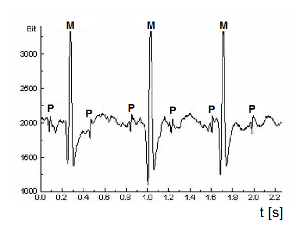
Figure 1.2 ECG of a pregnant woman: M – record of manifestation of depolarisation of the mother’s ventricular cells, P – record of manifestation of depolarisation of the foetus’s ventricular cells
Unlike the first above-mentioned component of time series, causes of origin of this parasitic component are mostly too complex; it is either unnecessary to search for its exact deterministic de-scription, or we might even not have relevant knowledge and skills. Description of the parasitic component is therefore usually based on general characteristics. Most mathematical tools for this way of description are derived from probability theory and statistics. However, there are also other tools to work with uncertain data, such as tools derived from fuzzy algebra or rough sets, deterministic chaos theory, fractal theory etc.
The basic problem in time series processing (and not only time series) is to separate the two components, i.e. to process the original data mix in a way that will provide pure data – not influenced by disturbances and related to the studied process only. All other problems are only extensions to this basic problem.
1.2 Parameters and properties of time series
1.2.1 Character of values
In general, values of time series y(ti) can take on both quantitative and qualitative. The vast majority of algorithms deal with processing of time series with quantitative values. We will also discuss these methods in the following chapters. Processing of time series with qualitative values employs somewhat different principles, mainly based on the automata theory.
Example:
Suppose we want to study a person’s relationship to smoking. We might introduce the following categories, for example:
N – non-smoker; S1 – occasional smoker (1–5 cigarettes per week); S2 – light smoker (1–5 cigarettes per day); S3 – moderate smoker (6–20 cigarettes per day); S4 – heavy smoker (more than 20 cigarettes per day); FS – former smoker. The sequence of values {N S1 S1 S3 S4 S4 S4 S4 S4 S3 S4 S2 FS} then describes the smoker’s changes in time.
A similar approach can be applied to categories such as unmarried, married, divorced, widower/widow.
The following text will only deal with the processing of time series of quantitative variables, such as the time series representing the year-on-year increase in retail sales in 2016 in the Czech Republic (Figure 1.3).
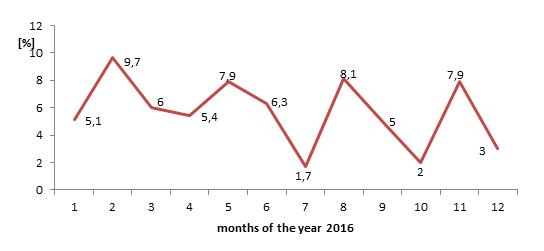
Figure 1.3 Year-on-year increase in retail sales in individual months of the year 2016 in the Czech Republic
1.2.2 Sampling
Time points ti might be distributed regularly or irregularly on the time axis. However, sampling (i.e. the process of determining the values of individual samples) must meet the so-called sampling theorem in both cases.
At this point, we should at least shortly mention that the mean frequency of sample occurrence must be at least double when compared to the maximum frequency of the harmonic component, which is part of the analysed variable.
Figure 1.4 demonstrates how the character of time series changes with different sampling frequencies. Annual sampling shows only basic trends in incidence and mortality rates of a given disease, whereas monthly sampling also reveals development in individual years.
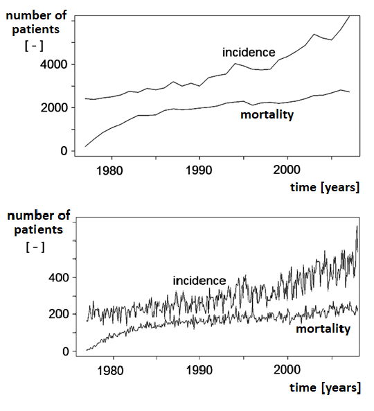
Figure 1.4 Trends in breast cancer incidence and mortality in the Czech Republic: (a) annual sampling, (b) monthly sampling.
Sampling regularity – or irregularity – is one of the basic properties which determine the way of time series processing. The following text will deal with methods of processing of regularly sampled time series.
More details on the sampling theorem, and on the consequences of respecting or non-respecting it, are provided in Chapter 3.
1.2.3 Number of channels – simultaneously recorded variables
In order to meet any objective that deals with time series, it is useful to have as much as possible information on both the subject (which is the source of variables to be processed) and its environment (in which this subject is located and is active ).
The first option of how to obtain more data on the behaviour of a given subject – or its environment – is to record multiple variables simultaneously. This type of data recording is referred to as multichannel or multicomponent in technical disciplines, whereas non-technical disciplines (such as economics or epidemiology) use the term panel data. Time series can be represented either by variables with the same units (Figure 1.5) or by different variables (Figure 1.6). The latter case is more frequent if the variables characterise the subject of interest and its environment (Figure 1.7).

Figure 1.5 Recording of a multichannel EEG signal. Individual curves represent the voltage generated by neurons and recorded in different positions on the skull.

Figure 1.6 Parallel recording of variables describing the heart’s activity: (a) and (b) phonocardiogram recorded in two positions on the chest; (c) ECG signal; (d) M-mode ultrasound – the horizontal axis again represents the time axis, whereas the vertical axis describes the depth of location of individual structures in the chest (the abbreviation MVE and arrows indicate movements of the mitral valve)
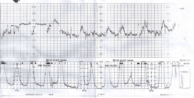
Figure 1.7 Cardiotocogram – the upper curve represents the foetus’s heart rate, whereas the lower curve represents the simultaneously recorded intensity of uterine contractions. This example points out the difficulty of distinguishing between the subject and its environment. Both curves might represent a single subject (mother together with the foetus) or describe the foetus’s reactions (or more precisely, reactions of the foetus’s cardiovascular system) to stimuli from the environment (uterine contractions).
1.2.4 Number of samples
The number of samples in a time series N is also one of the factors that determine the quantity and quality of information on data source. The larger number of samples in a time series, the more information on the subject of interest is contained.
The way of processing a time series is indirectly determined by the number of samples, i.e. the amount of available information. If the number of samples is low (up to about 20 samples), then the amount of a priori information about the subject of research and about the problem to be solved should be as large as possible, otherwise conclusions could not be considered reliable. In most cases, this a priori information contains pieces of information about the above-mentioned deterministic component of time series, which can be determined thanks to knowledge of the solved problem. This can be represented either by a specific mathematical description (a model) or by a more general idea on the monitored dependence. This information can also involve general assumptions on the non-deterministic component, such as the type of random variable distribution, the size of variance or other parameters (moments) of random variable etc.
1.3 Basic types of problems in time series processing
Problems to be solved in connection with time series fall into two basic categories: analysis of their properties and synthesis of their mathematical models. Both types of problems are usually very closely linked to each other.
1.3.1 Analysis
Decomposition to basic components – and the subsequent separation of individual components, if need be – is the main activity related to processing of any time series. Decomposition can be based either on the knowledge of processes involved in the origin of a given time series, or on theoretical – more or less blind – initial assumptions on its properties. The first case might be based on heuristic knowledge of a given process or on the mathematical description of individual components of the series.
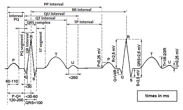
Figure 1.8 Schematic representation of parameters of ECG signal
ECG signal processing (Figure 1.8) is one example of heuristic decomposition. In this case, duration and height of waves, oscillations and intervals in a representative heart cycle in individual ECG leads are measured (physicians do it manually, whereas automated ECG is interpreted algorithmically). The knowledge of electrical processes in the heart – and their display on the ECG – determines which data are needed for a specific diagnosis. The final diagnosis is then established from these determined values.
Examples of the second situation involve all economic, biological, epidemiological and countless other phenomena which are repeated and which have a known repeating period (year, day, month, …). In theory and in practice, several basic types of time series components are distinguished:
- trend, expressing the monotonic tendency of development, the overall general tendency of long-term dynamics; let us call this component r(nTs), where Ts is the sampling period, i.e. the time difference between two consecutive samples.
- two basic types of deterministic oscillations according to period length: on the one hand, long-term oscillatory processes characterised by a period significantly longer than the duration of time series monitoring, let us call them z(nTs); on the other hand, the so-called seasonal components characterised by a period many times shorter than the duration of time series monitoring, let us call them s(nTs). A time series can involve multiple seasonal components; these can be produced by various processes. A trend combined with long-term oscillations is often called a drift.
- the noise component takes into account all deviations of time series samples from the course of deterministic part of the model, which are formed by the three above-mentioned components of time series; let us call it ν(nTs). Based on probability calculus, it is usually expected that the random noise component ν(nTs) of a time series represents the so-called white noise, which has a normal distribution, zero mean value and unit variance.
The analysis aims to define and subsequently to reveal individual component processes that form the resulting time series and to ascertain their partial influence on the final course of the series. The manner of separation is based on two basic models of time series structure: either additive or multiplicative. In the additive model, it is assumed that the values of samples of a time series are given by the sum
whereas in the multiplicative model, the values of samples of a time series are given by the product
There is an easy rule to decide which from the two models should be used, based on whether the magnitude of the periodic seasonal component depends on the instantaneous value of the trend. For example, the magnitude of oscillations in Figure 1.1 depends on the magnitude of the trend component; therefore, the multiplicative model can be used. By contrast, the magnitude of oscillations in foetal ECG in Figure 1.2 obviously does not depend on the magnitude of values of the trend (i.e., there is no obvious trend), suggesting that the simpler additive model should be rather used.
Apart from the two above-mentioned extreme cases of models, there are various mixed additive-multiplicative approaches.
The properties of disturbances and of useful components are sufficiently known (based on both experimental and theoretical knowledge) and a number of different algorithms for the separation of all components of time series to be analysed were developed. These algorithms use the principles of linear frequency filtering, statistical properties of both components in averaging, or other, more sophisticated approaches based on various transformations such as the wavelet transform, processing via neural networks etc. In this case, separation of individual components is based on the knowledge of their mathematical models.
The final way of time series decomposition is the decomposition to a set of sequences with defined properties, regardless of the a priori knowledge about the processed time series or about its source. This means that the time series is decomposed more or less blindly, or with just minimum requirements on the components of predefined waveforms. The Fourier transform is a standard example of this type of decomposition, decomposing any given time series to harmonic sequences with specified frequencies. The result of this decomposition is called a frequency spectrum. However, harmonic waveforms are not the only possibility. Binary sequences, taking on values 0 and 1, offer an easier calculation but a more complicated interpretation. In these sequences, time series can be decomposed by such a transform as the Walsh–Hadamard transform.
1.3.2 Synthesis
Development of a mathematical model for a specific time series not only contributes to our ability to understand the causes of its origin, but also makes it possible to estimate (to predict) its course beyond the interval in which values of the given time series are known: in future, in the past or in a time interval between two known waveforms. Moreover, individual components of time series can be classified according to values of parameters of corresponding models.
The methodology of model development can be either based on the knowledge of processes contributing to any given time series, or can rely on procedures requiring no a priori knowledge. In the latter case, the used methods can be divided into two basic groups, based on employed mathematical tools: methods using regression models and methods applying the theory of linear dynamical systems – either with constant parameters (determined by means of the Box-Jenkins method, for example) or with time-variant parameters (using different variants of adaptive systems). Regression models are important for the description of monitored events, whereas dynamical systems provide a better insight into the nature of these events.
1.4 Examples of time series processing
1.4.1 Classification
Classification is a typical problem to be solved in medical signal recordings, such as recordings of ECG or EEG signals (Figure 1.5). In these usually multichannel recordings, it is primarily necessary to separate the useful component of data from disturbances in all leads; these disturbances might be caused either by the activity of other parts of the organism (ECG – breathing, movement artefacts; EEG – eye movement) or by the outer environment (for example, induced voltage from the electricity distribution network). Furthermore, it is convenient to find relations between similar courses in individual leads of the recording and to localise potential sources of signal in this way. The filtered data can then be used to determine the values providing information necessary for the classification, and to establish the diagnosis.
1.4.2 Monitoring
Time series monitoring consists in the comparison of their values (preferably already cleared of parasitic disturbances) with predefined limit values. Exceeding these values signals an abnormal, undesirable or dangerous function of the monitored subject. Such monitoring is employed in medicine (when monitoring vital functions of patients in danger of death), in ecology (when monitoring environmental pollution), in economy (when monitoring the exchange rate of a currency), etc.
1.4.3 Modelling
Mathematical modelling of time series is the basic task that not only contributes to the understanding of processes in the subject of research and their relations (Figure 1.9); developed models can also serve as tools to separate individual components of data or even to estimate missing values.
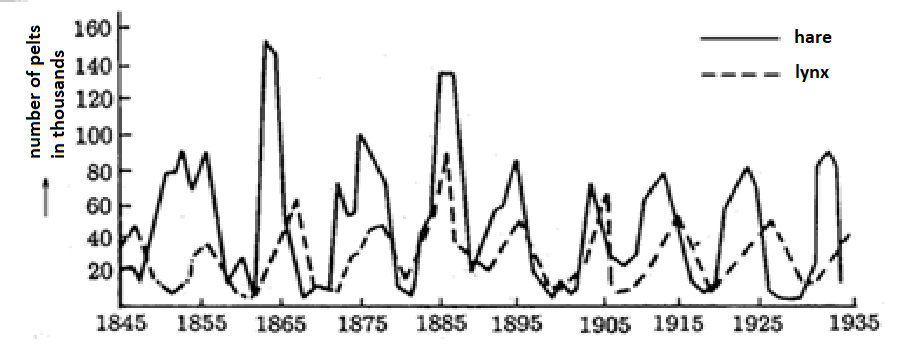
Figure 1.9 Numbers of pelts from Canada lynxes and snowshoe hares killed in the area of Hudson Bay between 1845 and 1935. The mathematical model of Lotka–Volterra for a two-species population of predator and prey supposes that the prey’s population curve precedes the predator’s population curve; however, mutual relations between the two curves do not meet this assumption in the entire monitored period (most notably in the period around 1885). True relations between both populations can be revealed by an analysis of the model’s non-functionality.
1.4.4 Prediction
Economic, epidemiological or demographic analyses, for instance (Figure 1.10), often need to estimate the behaviour of a monitored system in future, due to planning of organisational and financial requirements and effects. However, predictions of future behaviour usually cannot be solely based on the information contained in values of the respective time series, but also on many other additional pieces of information. One example is the sensitivity of the analysed subject to environmental influences or its own stability. Unlike demographic and epidemiological systems, economic systems are, by and large, much more sensitive to interventions from the environment, and their stability is more questionable, too. Because predictions of future development are based on mathematical models, it can be concluded that economic models will be much more complex and sophisticated.
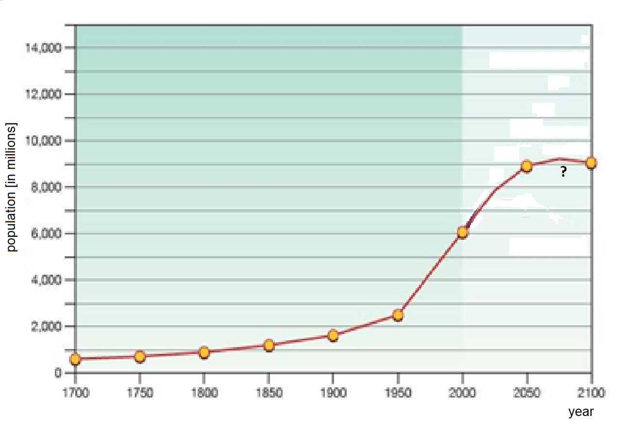
Figure 1.10 World population in the period 1700–2000 and predictions for the period 2000–2100 (According to UN Dept.Economic & Social Affairs Div., 2004)