Time Series Jiří Holčík
A linear system with input/output function y = f(x) is a system for which the superposition principle holds. The principle is defined by the two following formulas (see also Figure 5.2):

where c is a constant.
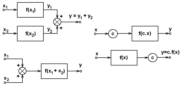
Figure 5.2 Schematic representation of relations defining superposition principle
The superposition principle is sometimes generally expressed in a form
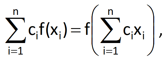
where ci are constants. The superposition principle can be generally interpreted as follows: if any complex problem is linear, then its solution can be obtained by a weighted sum of solutions of its individual components. Any system that does not meet the superposition principle, as indicated by Eq. (5.1) or Eq. (5.2), is non-linear.
Example:
Find out whether the systems with input/output functions depicted in Fig. 5.3 are linear.
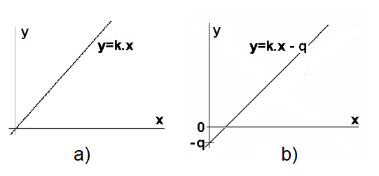
Figure 5.3 Examples of input/output functions – (a) linear function passing through the origin, b) linear function with intercept
Solution:
a)

where yL1 represents the computation according to the left side of the first definition of the superposition principle and yP1 represents the computation according to its right side, whereas yL2 represents the computation according to the left side of the second definition and yP2 represents the computation according to its right side. The system with input/output function according to Figure 5.3a meets the superposition principle and therefore is linear.
b)

The system with input/output function according to Figure 5.3b does not meet the superposition principle and therefore is not linear, although its input/output function has a linear character.
Chapter 5: Introduction to systems
5.1 System
The word “system” is frequently used in everyday language and we can all understand it without thinking too much about its precise meaning. We can say, for example, that “there was no system at all in the company”, meaning that there was no organised planning or behaviour (or orderliness).
Another example is a “cardiovascular system”. We understand this term, too, by knowing what such a system is composed of (e.g. the heart, arteries, veins, capillary bed, blood), how these individual parts are interconnected and how they work together. Only mutual connections and smooth cooperation among all components – or even their connection to the environment (something must control the cardiovascular system in order to make enough blood with required properties flow to locations where needed) – makes the cardiovascular system work how we know it. It would not work without blood, for example. Elements of the cardiovascular system are defined according to our point of view. For example, the heart can be thought of as a system consisting of the left and right atria and the left and right ventricles. Similarly, its vascular part can be divided into the systemic circulation and the pulmonary circulation.
The above-mentioned concept of system also applies to abstract systems used in mathematics, mainly for the model description of behaviour of real objects – systems. A system can therefore be defined as a set of elements linked by mutual connections into a meaningful whole, which outwardly manifests itself by a certain form of behaviour. This can be formally defined as follows.
Definition 5.1
A system S = {P, R} where P is a non-empty finite set of elements and R is a non-empty set of relations defined on P; both sets together determine the properties and behaviour of the whole.
The specific arrangement of elements and relations determines the internal structure of the system. The elements are basic components of the system, indivisible at a given resolution level. However, it does not necessarily mean that an element cannot have a different structure at another resolution level. Figure 5.1 shows that at a given level, the human organism can be divided into three basic components (elements): (1) information & control subsystem, (2) metabolism subsystem and (3) output units subsystem – although it is obvious that each of these elements (subsystems) actually consists of further components. This is schematically indicated in case of the information & control subsystem, which can be divided into genetical versus physiological subsystems. The physiological subsystem can be further divided into nervous system and endocrine system; furthermore, the nervous system can be divided into central nervous system and peripheral nervous system etc.
However, for the level determined by objectives of the analysis, the basic structure containing three elements is apparently sufficient.

Figure 5.1 Human organism as a system
Elements are described by variables defining their state or by other auxiliary variables. State variables are variables that unequivocally define the behaviour of elements and of the entire system. These variables represent cumulative processes within the system. The number of state variables determines the system order. State of an element – and of the system, too – is given by instantaneous values of variables at a given time. Depending on the development of state values, we distinguish static systems (there is no change in time) and dynamical systems. The behaviour of a system is determined by outward manifestations of the system and is a consequence of the system dynamics, i.e. of the ability to evoke changes in the system, mainly of the system state.
Relations are represented by connections either among individual system elements or between system elements and the system environment. The relations can be either energy-based (material) or information-based (immaterial). However, even an information-based relation must be obviously represented by a material variable. Particular relations are formally expressed by mathematical formulas that characterise connections among variables describing the state of elements; in graphical representation, mutual dependence of variables is given by the orientation of connecting links.
The system environment consists of elements that do not fall into the system but are connected to it. The system and its environment are partly objective facts, partly the consequence of subjective requirements on the contents, form and purpose of study. For example, when studying state of the environment in a certain location, a question arises whether pollution sources will be included in the system or whether they will be studied separately and their impact will then be thought of as system inputs for the analysed location. A similar situation can be met in a theoretical analysis of mathematical systems. Including the inputs in the system will often make analytical procedures easier.
The variables (relations) mediating environmental influences on the system are system inputs, whereas outward manifestations (relations) of the system, which represent the system influence on the environment, are system outputs. A system element that has a connection to the environment (either input or output, or both input and output) is called the boundary element of the system, and the set of all boundary elements is called the system border.
According to a relationship to the environment, we distinguish open and closed (conservative) systems. An open (non-autonomous) system is characterised by the possibility to exchange energy or information with its environment. By contrast, a closed (conservative, autonomous) system is isolated from its environment. From the practical point of view, we admit the existence of outputs providing information about the system state, otherwise we would not be able to find out (or to measure) the system’s instantaneous state.
The condition of system separability tells us whether we can include the environment (or its part) into the system or not. A system is separable if its outputs do not significantly influence inputs as a consequence of environmental influences.
Example:
The predator-prey model is one of the basic models of population dynamics, describing mutual relations between the hunting population and the population being hunted. The model uses two elements – the prey population and the predator population – which are characterised by their abundance or, alternatively, density. These are the state variables of this model, and the model/system is of second order. (We will see in the following chapter what that means from the viewpoint of mathematical description.) The system relations can be expressed by mathematical equations, describing how both populations influence each other and themselves. Because the model (as it is constructed) does not permit any of the two populations to be affected by any external influences, the system is closed/autonomous.
Pause for thought:
Can a football team be thought of as a system? If so, what are its elements and what variables would you use to describe its characteristics? What would be the system order? Would the system be autonomous or non-autonomous? How could its environment be described?
Stability is an important characteristic of the system. In general, stability can be defined as the system’s ability to maintain its outward form (behaviour) despite changing inputs and changing states of its elements, even despite very turbulent processes going on inside the system. Alternatively, it can be defined as the system’s ability to return to the original state after being deviated to a certain (not very large) extent.
If we are expected to work appropriately with the systems, i.e. to analyse their characteristics or to synthesise them (that means, to design their structure, based on specific requirements), we must be able to create their appropriate mathematical descriptions/models. Definition 5.1 is certainly mathematical enough, nevertheless, it is still not sufficiently applicable for practical problems. In this section, we could surely specify the above-mentioned definition for specific situation in more details. However, we will leave it to be discussed in later, more specifically focused chapters. Meanwhile, let us mention that mathematical tools for the description of systems can differ in:
- type of time base (continuous, discrete, time-independent);
- character of variables that the system works with (continuous, discrete, logical, nominal, ordinal) – in the context of this text, we will only deal with quantitative variables in subsequent paragraphs and chapters, assuming there are not significant differences between processing variables with continuous and discrete ranges;
- relation to its environment (autonomous, non-autonomous);
- variability of parameters (linear, non-linear, time-varying); relation to the past (without memory, with memory);
- determinism of variables and parameters (deterministic, non- deterministic – random, fuzzy, ...);
- requirements on the knowledge of internal structure of the system (outer or input/output description, state description).
Linearity and causality are other important characteristics of the system, mainly from the viewpoint of mathematical tools applicable to their analysis and to the synthesis of their models.
5.2 Linearity
A linear system with input/output function y = f(x) is a system for which the superposition principle holds. The principle is defined by the two following formulas (see also Figure 5.2):
where c is a constant.
Figure 5.2 Schematic representation of relations defining superposition principle
The superposition principle is sometimes generally expressed in a form
where ci are constants. The superposition principle can be generally interpreted as follows: if any complex problem is linear, then its solution can be obtained by a weighted sum of solutions of its individual components. Any system that does not meet the superposition principle, as indicated by Eq. (5.1) or Eq. (5.2), is non-linear.
Example:
Find out whether the systems with input/output functions depicted in Fig. 5.3 are linear.
Figure 5.3 Examples of input/output functions – (a) linear function passing through the origin, b) linear function with intercept
Solution:
a)
where yL1 represents the computation according to the left side of the first definition of the superposition principle and yP1 represents the computation according to its right side, whereas yL2 represents the computation according to the left side of the second definition and yP2 represents the computation according to its right side. The system with input/output function according to Figure 5.3a meets the superposition principle and therefore is linear.
b)
The system with input/output function according to Figure 5.3b does not meet the superposition principle and therefore is not linear, although its input/output function has a linear character.
5.3 Causality
In general, a causal system is a system of which output at each time point t0 only depends on the input variable for t ≤ t0. In other words, the value of output at each time only depends on the input at a given time and on the past of the input variable, not on its future. A system that does not meet this requirement is called a non-causal (or anticipatory) system. In another words, a system is causal if its output variable does not appears until the input variable is brought to the system input. As a matter of fact, all reasonable real systems are causal.
Time series usually start at a specific reference time, which is called the origin of time axis. Analogically, causal time series are time series for which x(n) = 0 for n < 0 (Figure 5.4).
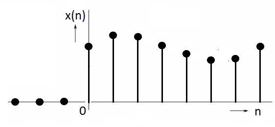
Figure 5.4 Causal time series
5.4 Final example to illustrate different types of systems
Example:
Let us illustrate the above-mentioned facts on a discrete model of a one-species population living in a certain region. Modelling the dynamics of one-species populations is based on a deterministic way of population behaviour; the state of a population is characterised by a number of its members.
Let us discuss several different situations:
a) autonomous linear system;
b) non-autonomous linear system;
c) autonomous non-linear system.
In all of these cases, there is a single element in the system/model of a one-species population. We will therefore deal with a first-order system in all the cases.
In general, in all of the above-mentioned cases, if s(n) is the number of individuals in the population at time n, then this value is given by the state of population s(n-1) in the previous time, which is however modified by processes going on in that population. The character of these processes then varies according to the below-mentioned situations.
Ad a) autonomous linear system
Because the system is not influenced by its environment, the dynamics of its behaviour only depends on its internal processes. Let them be determined by births of new individuals and by deaths of other individuals.
Suppose that the birth rate is determined by the so-called birth rate coefficient b, which is defined as the ratio of newly born individuals to all individuals in the population per a normalised sampling period (b ≥ 0 must hold for parameter b). Furthermore, the death rate is determined by the so-called death rate coefficient d, i.e. the ratio of individuals who died to all individuals in the population per a normalised sampling period (d ∈ <0; 1>). For a linear system, suppose furthermore that both coefficients are constant, independent of time or any other variable. Then the population dynamics can be expressed by a single constant parameter r = b – d, which can take on positive or negative values. And finally, suppose that we monitor the state of population continuously, starting from the origin of time axis (i.e. from time n = 0) in which s(0) – the initial value of the state of population – is known.
According to the definition of the birth rate coefficient, the number of newly born individuals in a time interval <n-1, n> is proportional to the state of population: sb(n) = b.s(n-1). Analogically, the number of individuals who died can be expressed as sd(n) = d.s(n-1). The difference equation describing behaviour of the defined system can be therefore written as
According to the difference equation constructed in this way, if the increment is zero (r = 0), the state of population in time n is equal to state of the previous generation, which corresponds to the expectation. However, if r = 0,5 (one offspring per two parents), the new state is equal to one and a half multiple of the previous generation. This corresponds to a situation when all individuals from the previous generation survive in the next generation and newly born individuals are added to it. A system defined in this way can be suitable as the model of a population where the lifespan of its members is longer than the maturing period, which is represented by the sampling step.
By substituting into Eq. (5.5) for s(n-1) according to the equivalent formula, we get
If we continue recursively, we get an expression to solve the defined difference equation based on the initial condition s(0)
This formula implies that the sequence {s(n)} grows exponentially for r > 0, decreases exponentially for r ∈ <-1, 0> and is constant for r = 0. The solution only depends on the values of parameters b and d (or r) and on the initial condition s(0). For r < -1, the sequence {s(n)} has an oscillatory character, with a changing polarity of its values; in fact, this has no practical meaning.
Ad b) non-autonomous linear system
In this case, the state sequence {s(n)} is dependent not only on the processes going on within the model population, but also on changes brought about by emigration to and immigration from the system environment. If we express the exchange of individuals in the system population with individuals in the environment by a single discrete variable x(n), which represents the difference between the number of individuals who emigrated to or immigrated from the environment during a time interval <n-1, n>, then the difference equation (5.5) can be written as follows:
The solution will then depend not only on the values of parameters b and d (or r), but on the input sequence x(n), too.
Ad c) autonomous non-linear system
Eq. (5.7) implies that the state sequence {s(n)} is exponential. If r > 0, it grows exponentially. However, there is only a limited space in which the population exists, and the same is true for the applicable energy. In real conditions, the population cannot grow infinitely. For this reason, let us modify the difference equation (5.5) in such a way that the death rate will depend on the population size instead of being constant: the larger population, the higher death rate. Consequently, let the parameter of death rate be defined by the formula d + c.s(n). Eq. (5.5) can be then rewritten as
where apart from the linear term, the state variable is also involved in the quadratic term. In this case, we are not able to determine the analytical solution of difference equation, as we were able to do it in the case of linear system. However, we can employ Eq. (5.9), the known value of s(n-1) and system parameters in order to determine the state of population in any subsequent time n.
If we considered a non-autonomous non-linear system, then, by analogy with Eq. (5.8), a term representing the input value would be added to Eq. (5.9):
and, after generalisation, we could write
or alternatively, after moving the respective variables to one side of the equation:
where p(s,n) is a system parameter which, in a non-linear system, generally depends on a system variable; in time-variant system, this parameter also depends on time. Because the parameter of a non-linear system is a function of state, which also depend on the system input in non-autonomous systems, characteristics of such systems are determined not only by its own structure (as in linear systems), but also depends on environmental influences.
Indeed, this fact is one of the main reasons for trying to analyse the behaviour of mathematical models (and thus to make the analysis easier) with elimination of environmental influences. This can be done, for example, by including the environment (as the source of data) in the system itself, which turns an originally open non-autonomous system into a closed system.
All of the above-mentioned examples imply that the system behaviour can be described by a difference equation of the same order as is the system order, i.e. the number of state variables. The form of difference equations in individual cases depends on the character of studied systems.
Pause for thought:
Try to use the superposition principle to prove the system linearity according to Eq. (5.5) and the system non-linearity according to Eq. (5.9).