Time Series Jiří Holčík
The Savitzky–Golay (S–G) filter is a discrete system/filter used for time series smoothing, i.e. for removing higher-frequency components of time series. In essence, the S–G filter has the characteristics of a low-pass filter, but the passband cutoff frequency is usually significantly higher than it is in the case of drift estimate.
Again, the S–G filter is essentially a moving-average filter, and therefore also a filter with finite impulse response. This time, the coefficients of impulse response are determined by the approximation of a time series segment by a polynomial function. It is therefore a kind of combination of polynomial approximation (described in Chapter 9) and filtering by a MA system.
Let us demonstrate the principle of computation of filter coefficient in an example where fivesample segments will be centrally approximated by a third-order polynomial. Some advantage of segments with odd numbers of samples were already explained in the discussion of phase characteristics; other advantages will become clear soon.
Suppose that we know values x(n+i), i= -2, -1, …, 2 in each interval of the time series. If we want to fit these five values in each interval of the time series with a cubic parabola, then coefficients of this parabola will be determined by minimisation of the total squared deviation between the actual value of each sample of the time series and its estimate, i.e. the expression

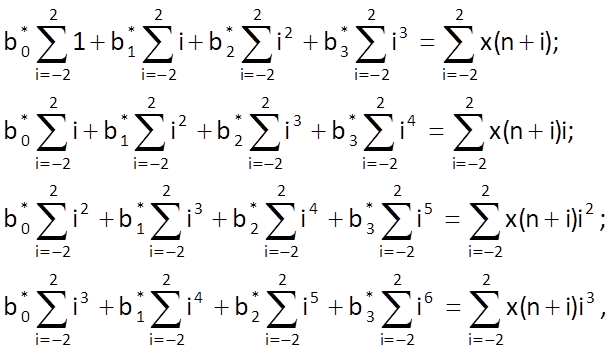
By deriving Eq. (10.37) according to parameters b0, …, b3, we get a system of four linear equations
As for individual values and their sums, we get
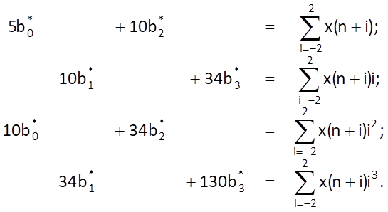
(Here is another, this time numerical, advantage of an odd number of samples of the explored interval, because ∑ij = 0 for any odd value of j and interval for i symmetrical about zero). Among all parameters b0*, …, b3* , only the value of b0* is useful for now, because it determines the estimate of time series value xe(n) in the middle of a given interval, i.e. for i = 0 (another advantage of an odd number of samples). Therefore, we only need to solve a system composed of the first and the third equation which, moreover, for one unknown, b0*, only . We can solve it by eliminating the parameter b2* , which leads to
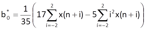
and, after writing out the sum terms, we get
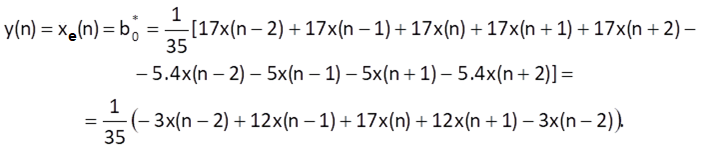
It means that weights for the computation of weighted average (and therefore also values for the filter impulse response) are {-3/35, 12/35, 17/35, 12/35, -3/35}. The impulse response is symmetric about the centre (that is, the filter has a linear phase response and does not introduce any phase distortion) and the sum of weights is equal to one (that is, the filter has a unit gain: it does neither amplify or attenuate input values). The filter frequency response is shown in Figure 10.14. The filter has the characteristics of a low-pass filter (the highest value of a transfer in the stopband is less than 10 dB) with a zero transfer at 3ωs/8.
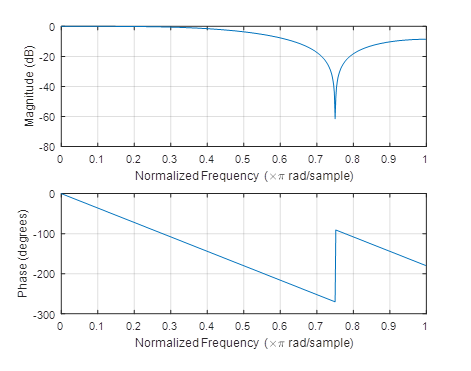
Figure 10.14 Frequency response of the Savitzky–Golay filter approximating a five-sample interval by a cubic parabola (in the range of frequencies up to half of the sampling frequency)
In general, we can design the Savitzky–Golay filter for a time series segment with a length of i = 2m+1 and an approximating polynomial of the r-th order. Apart from the above-mentioned characteristics (i.e. symmetry of the impulse response and the unit gain), it can also be demonstrated that weights of the impulse response and polynomials of the r-th order and the (r+1)-st order are identical (for example, it follows from the system of Eqs. (10.39) that the computation of parameter b0* does not depend on the value of b3*). The sample values for filter impulse responses for five- to thirteen-sample intervals and the polynomials of the third (or second) and the fifth (or fourth) order are shown in Table 10.4.
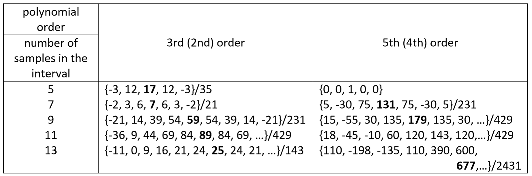
Table 10.4 Values of the impulse response of a S–G filter for various interval lengths and various orders of approximating polynomials (the middle sample of each sequence is marked in bold print)
Frequency responses of selected cases are shown in Figure 10.15. Figs. 10.15 and 10.14 imply that if the approximated interval is extended, the first lobe (the passband) becomes narrower; and if the order of the approximating polynomial increases, then the cut-off frequency of a passband (i.e. the width of the first lobe in the frequency response) becomes wider.
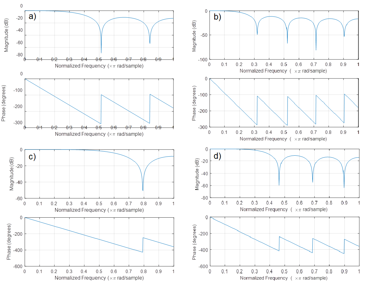
Figure 10.15 Frequency responses of selected S–G filters in the range of frequencies up to half of the sampling frequency: (a) third-order polynomial, interval length 7; (b) third-order polynomial, interval length 11; (c) fifth-order polynomial, interval length 7; (d) fifth-order polynomial, interval length 11 (in the range of frequencies up to half of the sampling frequency)
As it was the case in all MA systems, the problem of transient event at the beginning (and/or at the end) of the processed time series needs to be dealt with. Until now, we have solved this problem by setting initial (and/or terminal) conditions, which can surely also be applied in the case of a S–G filter. However, the S–G filter makes it possible to compute values of a transient event based on the knowledge of all parameters of the approximating polynomial. In the above-mentioned example, which we used to explain the principle of the method for a five-sample segment and a third-order approximating polynomial, we can determine the remaining parameters from the system of Eqs. (10.39) based on the following formulas:

Chapter 10: Frequency decomposition of time series
10.1 Introduction
In the preceding chapter, we looked into the separation of time series drift, i.e. the slowly changing component of a time series, using approximation methods. In this chapter, we will explain frequency filtering of other low-frequency components of a time series, i.e. not only the lowfrequency drift but also components with significantly higher frequencies. We saw in Chapter 8 that there are three basic computational structures for discrete-time systems, depending on the shape of transfer function:
- moving average (MA) systems;
- autoregressive (AR) systems
and, finally, if we connect the two structures serially, we will obtain
- autoregressive moving-average (ARMA) systems.
According to the Wold’s criterion (see Chapter 8), the computational structures are mutually interchangeable, with equivalent frequency characteristics.
The fundamental idea of transformation of an autoregressive system to a MA system (or vice versa) is based on the requirement of identity of their transfer functions. Therefore, we can write
which leads to
Here, let us suppose that the order q of the resulting MA system is much lower than the order of the original AR system. Because the convolution in the time domain corresponds to the product in the Z domain, we can write, based on Eq. (10.2):

Provided that p » q, we can estimate parameters bk more precisely using the method of the least squares. Each of the above-mentioned structures has its specific characteristics, advantages and disadvantages. Frequency characteristics that can be described by a low-order MA system will be expressed by an autoregressive system or, alternatively, by an ARMA system (usually of a significantly higher order) and vice versa. Parameters of an autoregressive system with required frequency characteristics or correlation characteristics can be computed relatively easily by solving a system of linear equations; impulse response of the MA systems can be determined from frequency requirements, using the relationship between the frequency response and the impulse response; and finally, MA systems can be designed (thanks to the finite number of samples in their impulse responses) in such a way that their phase frequency responses are linear, thus not introducing any phase distortion into the output sequence. Before we continue to explain the essential theoretical background, let us demonstrate in an example what impact various characteristics of a linear MA system have on a processed time series.
Example:
Suppose there is a time series {7, 9, 5, 4, 3, 9, 13, 8, 9, 13, 7, 5, 9, 13, 7, 6, 10, 6, 3, 6} (Figure 10.1). Figure 10.1 also shows the estimate of its mean value and the tolerance band determined by its standard deviation. Both the mean value and the tolerance band only describe the static characteristics of a time series. However, usually it is desirable to be able to express the dynamic characteristics of its components: the drift, which is not monotonic (increasing in the first half and decreasing in the second half of the time series), and two periodic components.
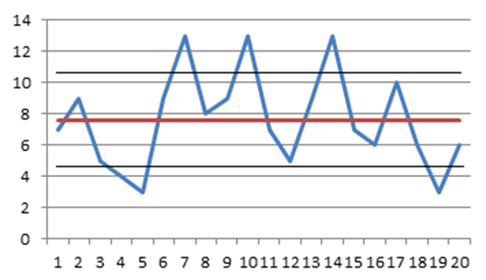
Figure 10.1 Time series and its mean value
Let us now try out how the shape of the above-given time series would change after passing through a MA system with a weighting sequence w(n) = {1/3, 1/3, 1/3}, n = 0, 1, 2. In the first case, we will use a causal system and our computation will be based on
(a procedure representing a standard computation in real-time digital signal processing), whereas in the second case, we will use a non-causal filter, which determines the output value of a sample in the middle of the applied interval/window according to following formula
(This computation, commonly used when solving economic problems, for example, determines the output sample in the centre of a computational interval. Both ways of computation have their theoretical interpretations, which we will see later.) Both the resulting time series are shown in Table 10.1 and in Figure 10.2. It is undoubtedly logical to expect that both output sequences would be mutually shifted by one sample and have the same shape with two waves. We can also see in the figure that number and location of values which cannot be computed depend on the computational algorithm: in case of a causal computation, two values at the beginning of the output sequence; and in case of a non-causal algorithm, one value at both the beginning and the end of the output sequence. If it is essential to maintain the length of a time series, then either initial conditions or terminal conditions must be used to complete the missing values, or the computational procedure must be modified.
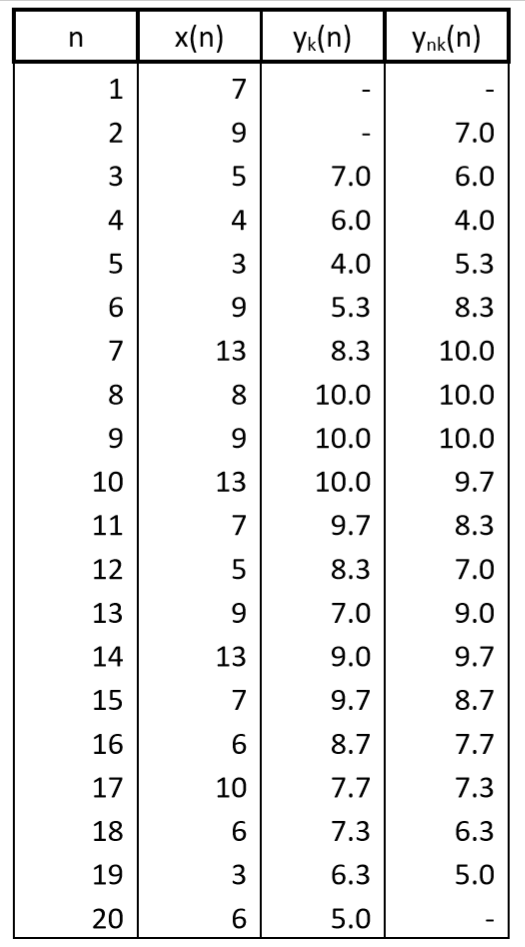
Table 10.1 Output values of a system with the weighting sequence w(n) = {1/3, 1/3, 1/3}
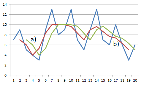
Figure 10.2 Time series filtered by a system with the weighting sequence w(n) = {1/3, 1/3, 1/3}: (a) causal system, (b) non-causal system
If initial conditions were equal to zero, i.e. x(-1) = x(-2) = 0, then in case of the causal computation, the initial segment of the output sequence would be {2,3; 5,3; 7,0; 6,0; 4,0; …} (Figure 10.3). It means that in fact the first output value y(0) would be determined by a formula y(0) = w(2).x(0), whereas the second one would be determined by y(1) = w(2).x(1) + w(1).x(0). In other words, the first two values of the output sequence would be temporarily determined by algorithms other than that mentioned in Eq. (10.4). The first part of an output sequence with a length M-1 (where M is the length of the weighting sequence), thus represents a temporary way of computation – or, a transient event at the beginning of the output sequence. In case of the non-causal computation, we must use the prerequisite for values not only before the processed segment of a time series, but also after its end. In this specific example of the above-mentioned time series, it was x(-1) = x(21) = 0.
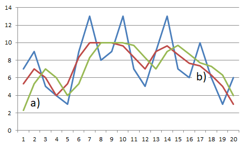
Figure 10.3 Shape of the input and output time series for a (a) causal or (b) non-causal MA system with a weighting sequence w(n) = {1/3, 1/3, 1/3} with zero initial and terminal conditions.
Now, let us modify the non-causal computation of output samples both by making the computational window longer and by changing the coefficients of the moving window. Let us consider a window with the length of seven samples and two different sets of the coefficients. The weighting sequence will be {1/7, 1/7, 1/7, 1/7, 1/7, 1/7, 1/7} in the first case (i.e. this will still involve the computation of average with uniform weights), and {1/7, -1/7, -1/7, 1/7, -1/7, -1/7, 1/7} in the second case. The resulting time series are shown in Table 10.2 and in Figure 10.4.
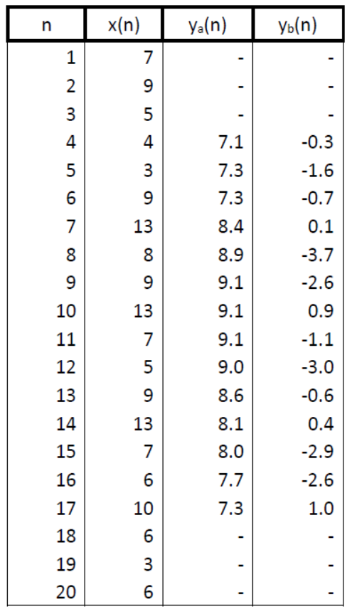
Table 10.2 Output values of non-causal systems with weighting sequences (a) wa(n) = {1/7, 1/7, 1/7, 1/7, 1/7, 1/7, 1/7} and (b) wb(n) = {1/7, -1/7, -1/7, 1/7, -1/7, -1/7, 1/7} with zero initial and terminal conditions
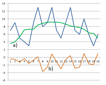
Figure 10.4 Time series filtered by non-causal systems with weighting sequences wa(n) = {1/7, 1/7, 1/7, 1/7, 1/7, 1/7, 1/7} a wb(n) = {1/7, -1/7, -1/7, 1/7, -1/7, -1/7, 1/7} with zero initial and terminal conditions
It is obvious from the shape of output sequences that the result of filtering can be significantly influenced just by the selection of coefficients of the weighting sequence. In the first case, i.e. the filter with a window with coefficients {1/7, 1/7, 1/7, 1/7, 1/7, 1/7, 1/7}, all oscillatory components were removed from the input sequence and the result represented the estimate of drift of the original time series. In the second case, by contrast, the drift was removed from the input time series and the resulting sequence represents oscillatory component of the highest-frequency in the input sequence.
The above-mentioned example demonstrates that the filter activity can be significantly influenced by the selection of the window length and its coefficients. The question is, how should the window length and the coefficients be set if we want the filter to meet our expectations? Shapes of the beginning and the end of the processed segment of time series represent another challenge to be solved.
10.2 Separating the drift of a time series by a MA system (or a FIR system)
10.2.1 Relationship between moving average systems and finite impulse response systems
The general formula to compute the response y(n) of a causal MA system to an input sequence x(n) is
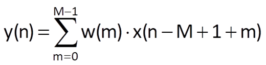
where w(m), m = 0, 1, 2, …, M-1 is the weighting sequence/window and x(•) is the input sequence of the system (Figure 10.5).
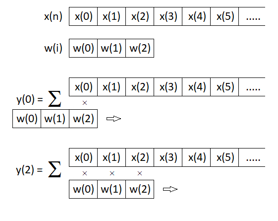
Figure 10.5 Computational diagram for the response of a causal MA system with a window of the length of three samples
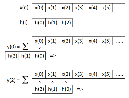
Figure 10.6 Computational diagram for the response of a causal linear system using convolution with a finite impulse response involving three samples
Chapter 2 introduced the convolution operation in the form of Eq. (2.38), which was graphically shown in Figure 2.15. Furthermore, convolution was used in Chapter 6 to compute the response of a causal linear system by Eq. (6.33), where one of the sequences entering the computation was the input sequence of a system x(n) and the second sequence was its impulse response h(m). The computational diagram for this case is graphically shown in Figure 10.6. The comparison of defining equations and diagrams shown in Figures 10.5 and 10.6 implies that both procedures are identical if samples of the weighting function (given by values of the finite impulse response) enter the computation in an inverse order. If the weighting function (impulse response) is symmetrical about the centre, both computational algorithms are entirely equivalent.
10.2.2 Basic characteristics of MA systems/ FIR systems
First, let us repeat and then extend the basic findings about the characteristics of moving average systems and finite impulse response systems, which are basically identical, as we have demonstrated in the preceding section.
If the impulse response of a linear system is h(n) = {h(0), h(1), …, h(M-1)}, its transfer function is given by its Z-transform (Chapter 6, Eq. (6.31))
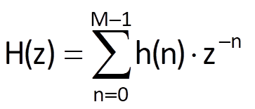
After substituting z = eiΩTs, where Ts is the sampling period, Eq. (10.7) gives the frequency transfer function
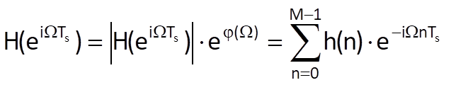
Taking into account the periodicity of function eiωTs with a period equal to the angular sampling frequency ωs=2π/Ts, it follows that the frequency transfer function is also periodic (with the same period).
Now, let us look into the characteristics of function ϕ(Ω), which determines the shape of the phase frequency response of the system. Due to the properties of a complex exponential function, this function is odd, i.e. we can write ϕ(-Ω) = - ϕ(Ω). Furthermore, this function is generally nonlinear; from the point of view of quality of the output sequence of the system, however, a linear phase frequency response would be more convenient, i.e. we would like the following to hold:
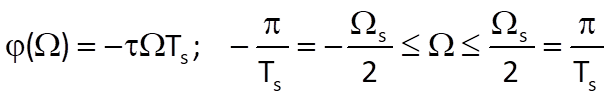
where τ is a constant determining by how many samples the system’s output is delayed when compared to the input sequence. In that case, the system does not introduce the so-called phase distortion – during processing, the delay of all harmonic components is directly proportional to their frequencies (Figure 10.7).
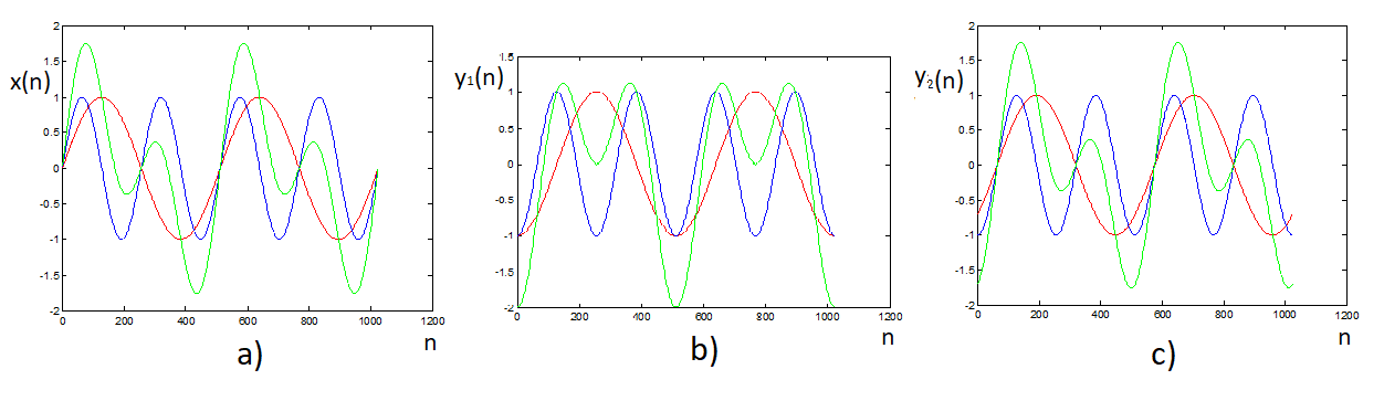
Figure 10.7 Phase delay influence on the sequence shape (the resulting green curve is composed of two component curves; frequency of the blue curve is two times higher than frequency of the red curve) – (a) original shape; (b) both component sequences have an equal delay ϕ1 = ϕ2 = π/2; (c) the phase delay of both components is proportional to their frequencies ϕ1 = π/4; ϕ2 = π/2 – the resulting curve is delayed compared to the original, but its shape has remained the same
The question is whether the shape of weighting function/impulse response has any influence on the shape of phase frequency response.
If the phase frequency response is linear (i.e. ϕ(Ω) = -τΩTs), then Eq. (10.8) can be rewritten into the form
Because eiα = cosα + i.sinα, the equality of complex values in Eq. (10.10) can be expressed by the equality of their real and imaginary parts
Considering the ratio of both equations
After multiplication of both sides of the equation by their denominators we obtain
and then
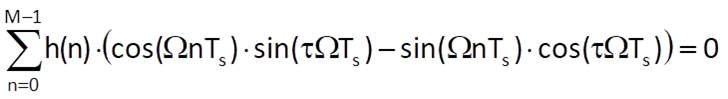
If we take into account the formula sin(α-β) = sinα.cosβ – cosα.sinβ, we can write the equation
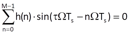
which has the solution
only if
i.e. if its impulse response is symmetric. In that case, we can expand Eq. (10.14) into the form

and
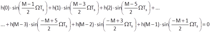
Because sine is an odd function, i.e. sin(-α) = -sin(α), Eq. (10.17) is certainly true if the condition (10.16) for the symmetry of impulse response is met.
There are two types of symmetric sequences for either an odd or an even number of samples (Figure 10.8). In case of a finite impulse response with an even number of samples, the value τ is not an integer number: the axis of symmetry runs between the (M/2-1)th sample and the (M/2)th sample. If there is an odd number of samples in the impulse response, the axis of symmetry runs exactly through the [(M-1)/2]th sample and τ = (M-1)/2 is an integer. This is the reason why the impulse response with an odd number of samples is more preferable in most of cases.
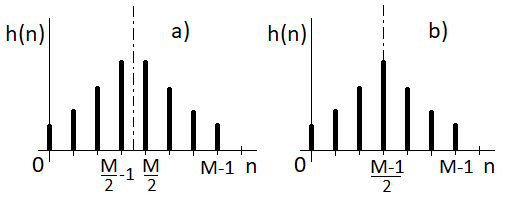
Figure 10.8 Finite impulse response with (a) an even number of samples and (b) an odd number of samples
Considering the system with an odd number of samples, if we shift the axis of symmetry into the origin of time axis, then τ = 0 – i.e. passing through the system does not formally introduce any delay. In that case, non-zero values of impulse response must be h(n) = {h[-(M-1)/2], h[-(M-3)/2], …,h(-1), h(0), h(1), …, h[(M-3)/2], h[(M-1)/2]}. That means that the system is not causal – you would need to know future samples of the input sequence to compute its response using the convolution. The Z-transform (which must be bilateral for non-causal system) of impulse response, i.e. the transfer function, is
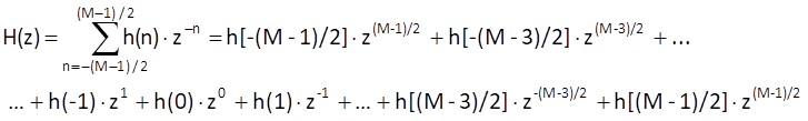
and therefore, we can write the following for the frequency transfer function

![]()
Provided that the impulse response is symmetric, i.e. h(n) = h(-n), for n = 1, 2, …, (M-1)/2, Eq. (10.19) can be rewritten into the form

And, because the following equation holds
here is the resulting equation for the frequency transfer function of a non-causal system with a symmetric impulse response, an odd number of samples and a centre in the origin of time axis:
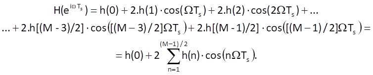
Because all summation terms in Eq. (10.21) are real, the phase function is ϕ(Ω) ≡ 0, which obviously corresponds to the presumption that τ = 0, i.e. that processing a time series by this system does not introduce any delay. This also explains the behaviour of the non-causal filter shown in the example in section 10.1.
10.2.3 MA system with uniform weights
At this moment, we still put emphasis on the elimination of drift of a time series (i.e. its lowfrequency components), although as a matter of principle, our aim is to separate all the time series components with different frequencies. The width of passband (if drift estimate is the expected result of separation) or the width of stopband (if time series shape without drift is the expected result of separation) must be estimated from the frequency spectrum of the processed time series.
A low-frequency component of a time series can be most easily estimated by a moving average system with uniform weights. In this case, the impulse response is defined (in a non-causal representation) as
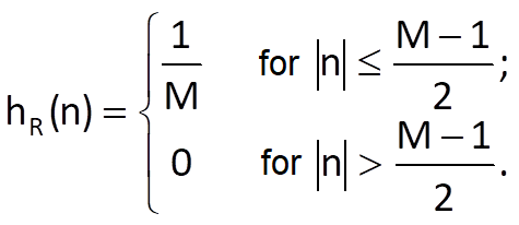
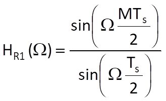
The frequency transfer function of a sequence hR(n) is
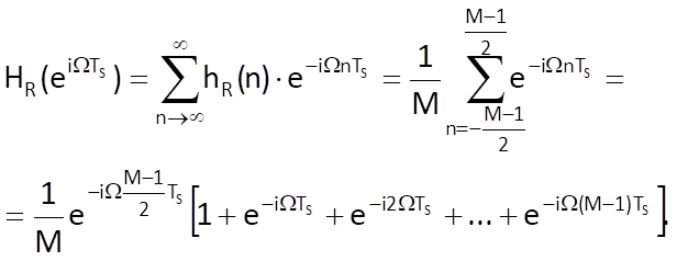
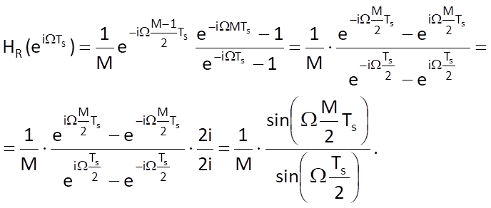
The sum of M terms of a geometric series in the bracket with the first term equal to one and with the quotient q = e-iΩTs is (e-iΩMTs – 1)/(e-iΩTs - 1) . As for the frequency transfer function, we can therefore write:
Note
The shape of frequency transfer function according to Eq. (10.24) is somewhat different from the shape of spectral function sin(x)/x, which was determined in Chapter 3 for the rectangular shape of time function. This difference is one of the consequences of sampling and the resulting periodisation of spectral functions.
For the above-given shape of impulse response, the function HR(eiΩTs) is a real periodic function of a continuous variable Ω with a period Ωs = 2π/Ts (see Figure 10.9 as an example).
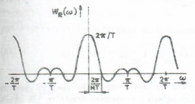
Figure 10.9 Example of a shape of the frequency transfer function of a MA system with uniform weights
The function passes through zero if the argument of sine function in the numerator is equal to integer multiples of π, i.e. ΩkMTs/2 = kπ. Therefore, frequencies where HR(eiΩTs) passes through zero are given by Ωk = 2kπ/MTs = kΩk/M. These frequencies are therefore inversely proportional to the length of impulse response. The function passes through zero for the first time at Ω1 = Ωs/M. This frequency can be approximately thought of as the passband cutoff frequency for a filter which lets pass through low-frequency components, the so-called low-pass filter. The longer the impulse response, the narrower the passband cutoff frequency. There are additional extremes between the frequency Ω1 and the half of sampling frequency Ωs/2, the so-called side lobes. As we will see further in this text, various applied weighting sequences of a given length differ in their passband widths and in sizes of their side lobes in the stopband. Among the known weighting sequences, the weighting sequence with uniform weights has the narrowest passband and, unfortunately, the highest side lobes.
Note
When processing various (not only economic) time series, it is necessary to use a weighting window with an even number of samples to smooth data (i.e. to estimate the drift) when averaging yearly data obtained by quarterly or monthly sampling. As we mentioned earlier, when there is an even number of samples, there is such a phase shift that the computed value corresponds to a time between two samples (see Figure 10.8). This problem is solved by a subsequent averaging of two neighbouring moving averages.
Let us consider the averaging of quarterly data as an example:
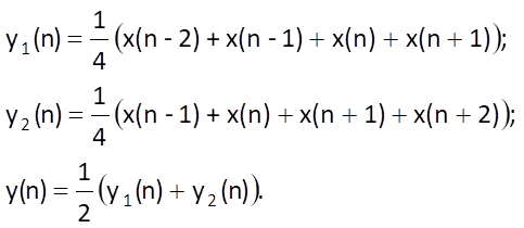
Combination of the above-mentioned equations leads to an algorithm which represents a non-causal averaging of an odd number of centrally located samples (i.e. with a zero phase shift), but with nonuniform weights:
How can this heuristic procedure be interpreted from the point of view of the abovementioned theory? The Z-transform of Eqs. (10.25) leads to
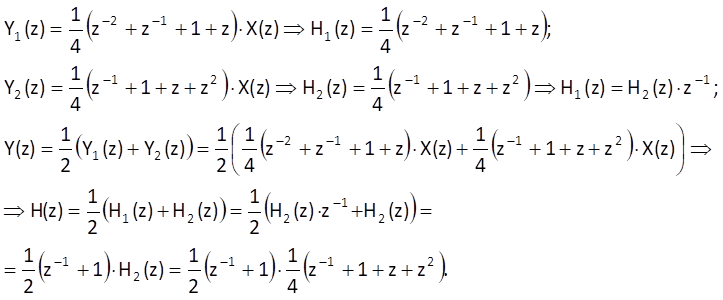
It follows that the computation according to Eq. (10.26) can be expressed by a serial connection of a linear causal system with an impulse response h1(n) = {0.5; 0.5}, n = 0,1 and a noncausal system with an impulse response h2(n) = {0.25; 0.25; 0.25; 0.25}, n = -2, -1, 0, 1. Magnitude frequency responses of both component systems and the resulting system are shown in Figure 10.10.

Figure 10.10 Magnitude frequency responses of component systems and the resulting system according to Eqs. (10.27) – characteristics for impulse response (a) h(n) = {0.5; 0.5}, (b) h(n) = {0.25; 0.25; 0.25; 0.25}, (c) characteristic of the resulting system
Example:
Let us determine the order of a discrete system with a finite impulse response and with uniform weights to estimate the shape of drift of the basic line of a time series, provided that data sampling is weekly and that the minimum period of drift fluctuation is one month, i.e. four weeks.
Solution:
The angular frequency at which the function passes through zero for the first time – i.e. the cutoff angular frequency for the low passband – can be determined from the above-mentioned formula Ω1 = Ωs/M. The number of samples of the impulse response is then M = Ωs/Ω1 = fs/f1. Provided that the reference time unit is one year, then fs ≅ 52 samples/year and the maximum frequency of fluctuation corresponds to 13 samples/period, i.e. f1 = 52/13 = 4 cycles/year. Then, according to the above-mentioned formula, M = 52/4 = 13. The magnitude frequency response and the phase frequency response of the filter mentioned in this example in a normalised frequency range (from zero to half of the sampling frequency) are shown in Figure 10.11.
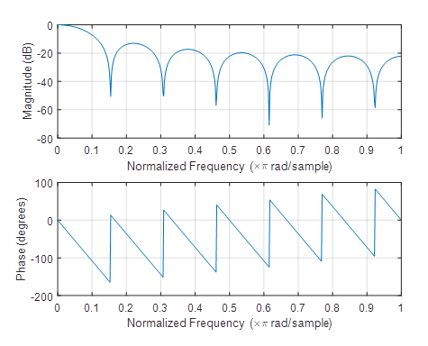
Figure 10.11 Frequency responses of the filter mentioned in this example
If our objective is to obtain the time series waveform without drift, the estimated drift can be subtracted from the input sequence. However, the input sequence must be delayed by τ = (M-1)/2 samples, which is the delay caused by passage of the time series through the low-pass FIR filter. The computational diagram for this case is shown in Figure 10.12.
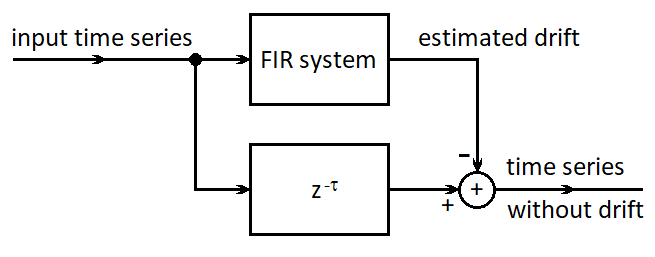
Figure 10.12 Computational scheme for filtering the drift from the input time series
10.2.4 MA systems with non-uniform weights
There are many other weighting functions that can be used for the construction of systems which make it possible to estimate the shape of low-frequency component of a time series.
Note
Besides the above-mentioned purpose, these weighting functions are also used in various other applications. Methods for the estimation of frequency spectra are one of possible examples.
Apart from the already mentioned sequence with uniform weights, the following weighting sequences can be thought of as classic weighting functions:
- triangular (Bartlett, Feier)
- Hamming;
- Blackman;
- cosine power sequences.
These weighting sequences are relatively simply defined in the time domain but have not very favourable spectral characteristics (in terms of steepness or ripples in magnitude frequency responses). That is why some additional sequences were derived, which have more favourable spectral characteristics but are incomparably more difficult to compute. Kaiser window, Dolph-Chebyshev window, kernel sequences (and a few others) can be given as examples of such weighting sequences.
Triangular weighting sequence
The triangular weighting sequence is defined as
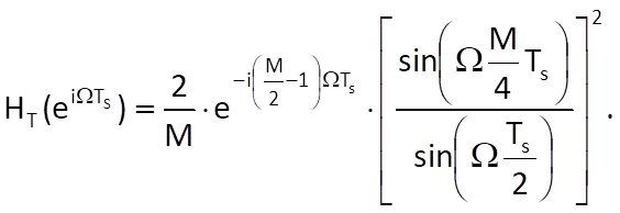
and its spectral function is
Hamming weighting sequence
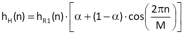
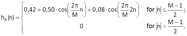
The generalised Hamming sequence is determined by

where α is a constant, generally from the interval 〈0, 1〉. When α = 25/46 (α ≅ 0,543478261), the first side lobe of the spectral function is suppressed to its minimum; its spectral function can be determined as a result of the following reasoning.
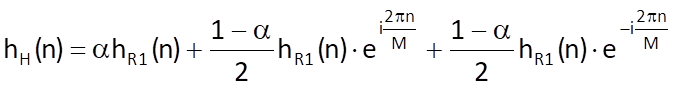
The sequence defined by Eq. (10.30) can be understood as a product of the weighting sequence with M unit weights hR1(n) and an infinitely long sequence hH(n) for n ∈ (- ꝏ , ꝏ ). In that case, we can write
After writing out the cosine function according to the Euler’s formula, we get
The spectral function for the Hamming sequence can now be comfortably established from the previously determined spectral function for a weighting sequence with uniform weights:
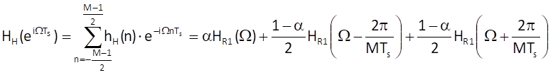
where
is the so-called Dirichlet function.
Blackman weighting sequence
The Blackman weighting sequence is defined by
Shape of the above-mentioned weighting sequences and their spectral functions are shown in Figure 10.13.
Cosine weighting sequence
The cosine weighting sequences are defined for various powers, usually from the first to the fourth. For the second power, the cosine sequence – the so-called Hanning sequence – is defined as
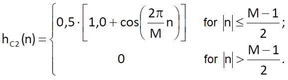
and its spectral representation is

where D(Ω) = eiΩTs/2.HR1(Ω).
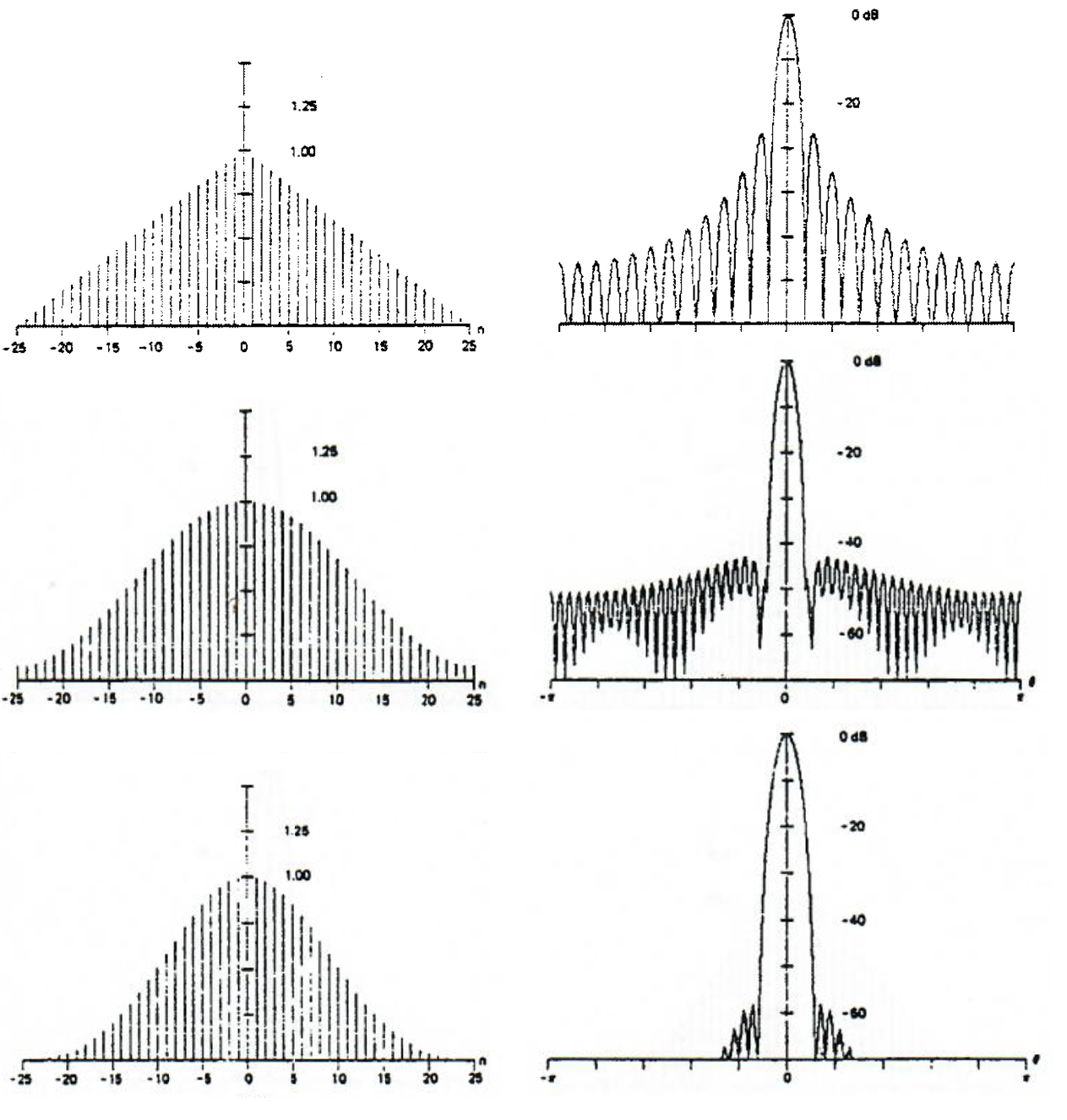
Figure 10.13 Weighting sequences and their spectral functions: (a) triangular weighting sequence, (b) Hamming weighting sequence, (c) Blackman weighting sequence (according to Harris, F.: On the Use of Windows for Harmonic Analysis with the Discrete Fourier Transform. Proc.IEEE, vol.66, Jan 1978, p.51-83)
The comparison of basic characteristics (i.e. widths of the main lobe of spectral function and size of the first side lobe compared to the main lobe of spectral function) is shown in Table 10.3.
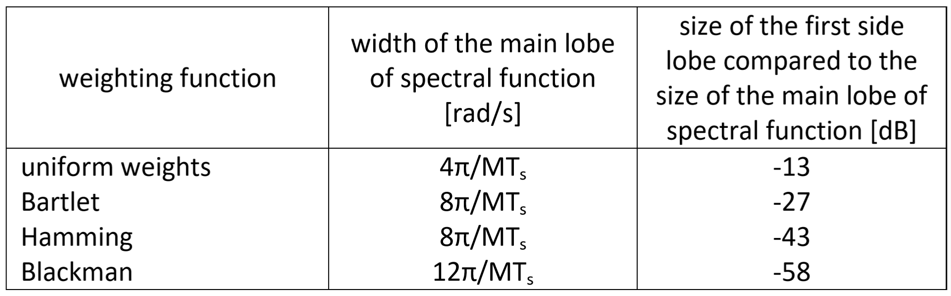
Table 10.3 Basic characteristics of four basic MA systems
10.3 Savitzky-Golay filter
The Savitzky–Golay (S–G) filter is a discrete system/filter used for time series smoothing, i.e. for removing higher-frequency components of time series. In essence, the S–G filter has the characteristics of a low-pass filter, but the passband cutoff frequency is usually significantly higher than it is in the case of drift estimate.
Again, the S–G filter is essentially a moving-average filter, and therefore also a filter with finite impulse response. This time, the coefficients of impulse response are determined by the approximation of a time series segment by a polynomial function. It is therefore a kind of combination of polynomial approximation (described in Chapter 9) and filtering by a MA system.
Let us demonstrate the principle of computation of filter coefficient in an example where fivesample segments will be centrally approximated by a third-order polynomial. Some advantage of segments with odd numbers of samples were already explained in the discussion of phase characteristics; other advantages will become clear soon.
Suppose that we know values x(n+i), i= -2, -1, …, 2 in each interval of the time series. If we want to fit these five values in each interval of the time series with a cubic parabola, then coefficients of this parabola will be determined by minimisation of the total squared deviation between the actual value of each sample of the time series and its estimate, i.e. the expression
By deriving Eq. (10.37) according to parameters b0, …, b3, we get a system of four linear equations
As for individual values and their sums, we get
(Here is another, this time numerical, advantage of an odd number of samples of the explored interval, because ∑ij = 0 for any odd value of j and interval for i symmetrical about zero). Among all parameters b0*, …, b3* , only the value of b0* is useful for now, because it determines the estimate of time series value xe(n) in the middle of a given interval, i.e. for i = 0 (another advantage of an odd number of samples). Therefore, we only need to solve a system composed of the first and the third equation which, moreover, for one unknown, b0*, only . We can solve it by eliminating the parameter b2* , which leads to
and, after writing out the sum terms, we get
It means that weights for the computation of weighted average (and therefore also values for the filter impulse response) are {-3/35, 12/35, 17/35, 12/35, -3/35}. The impulse response is symmetric about the centre (that is, the filter has a linear phase response and does not introduce any phase distortion) and the sum of weights is equal to one (that is, the filter has a unit gain: it does neither amplify or attenuate input values). The filter frequency response is shown in Figure 10.14. The filter has the characteristics of a low-pass filter (the highest value of a transfer in the stopband is less than 10 dB) with a zero transfer at 3ωs/8.
Figure 10.14 Frequency response of the Savitzky–Golay filter approximating a five-sample interval by a cubic parabola (in the range of frequencies up to half of the sampling frequency)
In general, we can design the Savitzky–Golay filter for a time series segment with a length of i = 2m+1 and an approximating polynomial of the r-th order. Apart from the above-mentioned characteristics (i.e. symmetry of the impulse response and the unit gain), it can also be demonstrated that weights of the impulse response and polynomials of the r-th order and the (r+1)-st order are identical (for example, it follows from the system of Eqs. (10.39) that the computation of parameter b0* does not depend on the value of b3*). The sample values for filter impulse responses for five- to thirteen-sample intervals and the polynomials of the third (or second) and the fifth (or fourth) order are shown in Table 10.4.
Table 10.4 Values of the impulse response of a S–G filter for various interval lengths and various orders of approximating polynomials (the middle sample of each sequence is marked in bold print)
Frequency responses of selected cases are shown in Figure 10.15. Figs. 10.15 and 10.14 imply that if the approximated interval is extended, the first lobe (the passband) becomes narrower; and if the order of the approximating polynomial increases, then the cut-off frequency of a passband (i.e. the width of the first lobe in the frequency response) becomes wider.
Figure 10.15 Frequency responses of selected S–G filters in the range of frequencies up to half of the sampling frequency: (a) third-order polynomial, interval length 7; (b) third-order polynomial, interval length 11; (c) fifth-order polynomial, interval length 7; (d) fifth-order polynomial, interval length 11 (in the range of frequencies up to half of the sampling frequency)
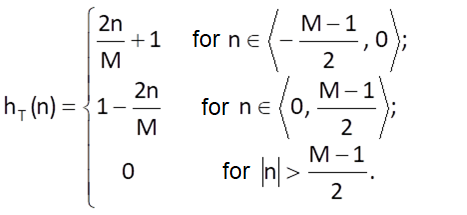
As it was the case in all MA systems, the problem of transient event at the beginning (and/or at the end) of the processed time series needs to be dealt with. Until now, we have solved this problem by setting initial (and/or terminal) conditions, which can surely also be applied in the case of a S–G filter. However, the S–G filter makes it possible to compute values of a transient event based on the knowledge of all parameters of the approximating polynomial. In the above-mentioned example, which we used to explain the principle of the method for a five-sample segment and a third-order approximating polynomial, we can determine the remaining parameters from the system of Eqs. (10.39) based on the following formulas: