Time Series Jiří Holčík
We have started the decomposition of continuous functions to harmonic functions by a decomposition of periodic functions using the Fourier series. We going to skip this first step in this chapter dealing with discrete sequences, and we will use it later in a computation of frequency spectra of time series with finite lengths.
Chapter 4: Frequency spectra of time series
4.1 Introduction
We have started the decomposition of continuous functions to harmonic functions by a decomposition of periodic functions using the Fourier series. We going to skip this first step in this chapter dealing with discrete sequences, and we will use it later in a computation of frequency spectra of time series with finite lengths.
4.2 Decomposition of discrete sequences to basic components – discrete-time Fourier transform
Provided that we know the function over the entire time interval for t ∈ (- ꝏ, ꝏ), we can write the following formula for the Fourier transform of a time-continuous non-periodic function x(t), according to Eq. (3.13) from the preceding chapter:

whereas the following formula holds for an inverse Fourier transform, making it possible to compute the original function (see Eq. (3.12)):

An equivalent formula is valid also for a time series which resulted from an original time-continuous variable with a limited spectrum by regular sampling with a sampling period Ts and provided that the sampling theorem was met. This is the so-called discrete-time Fourier transform (DTFT):
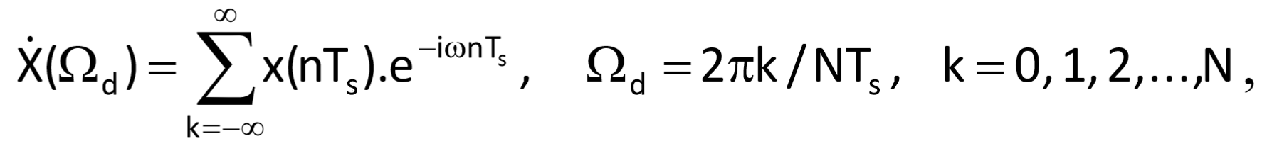
where Ωd for N → ꝏ is a continuous (non-discrete) variable.
The above-mentioned formula confirms what we already know from the decomposition of continuous function: the continuity or discontinuity of a spectrum is not related to the continuity or discontinuity of the function to be decomposed; rather, it is related to its periodicity. Furthermore, let us remind you that due to sampling, the spectral function X(Ωd) is periodic with a period equal to the angular sampling frequency, i.e. ωs= 2π/Ts.
Due to continuity of X(Ωd) in the frequency domain, the inverse computation of a time series is given by the following integral formula:
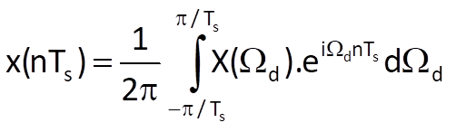
integrated over one spectral period, i.e. over the interval <-ωs/2; ωs/2>.
4.3 Discrete Fourier transform (DFT)
It is convenient to discretise the spectral function in order to be able to use the frequency spectrum in practical computations. Moreover, practical problems always suppose that there is a finite number of samples in the original time series.
Definition 4.1
Let us suppose that the sequence x(nTs) is finite and that it contains N samples. This means that x(nTs) = 0 for n < 0 and n ≥ N; DFT is then defined as

The inverse discrete Fourier transform is then defined as

If we consider only a sequence of values without its time interpretation or frequency interpretation, the definition for a discrete Fourier transform can also be defined in the form

or alternatively, here is the formula for the inverse transform:

It is valid that
This property of a discrete Fourier transform is called the invertibility. It can be proved as follows:
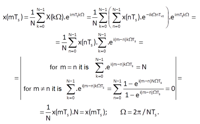

Figure 4.1 Principle and consequences of the discrete Fourier transform (DFT) for a frequency ω1 = ωs/4 = π/(2Ts) (based on Jan,J.: Diskrétní metody zpracování biosignálů. Praha, SNTL 1976)
The influence of the DFT on the character of spectrum of a harmonic sequence is apparent from Figures 4.1 and 4.2. Figure 4.1 shows a case where the period of sampled function T = 2π/ω1 is equal to an integer multiple of sampling period Ts = 2π/ωs, specifically T = 4Ts, i.e. ω1 = = ωs/4 = π/(2Ts). Both figures (4.1) and (4.2) show time representation on the left and corresponding spectra on the right. The finite interval of a function is created from its original, time-unlimited function by its multiplication by a rectangular window the length of which is equal to an integer multiple of the sampling period, specifically N = 8. Spectrum of the multiplied, i.e. time-limited interval of a continuous harmonic function is given by a convolution of spectra of the original harmonic function and the spectrum of rectangular window in the form of function Sa(ω). According to the definition (Eq. (3.41)), sampling this finite interval of an original harmonic function is expressed by multiplication by a train of unit impulses with period equal to the sampling period Ts. This also corresponds to a periodic impulse spectrum with a period equal to the sampling frequency ωs = NΩ; therefore, the resulting spectrum of the sampled sequence is given by the convolution of all three components, which were multiplied to provide a discrete harmonic sequence with a limited duration.
We get the discrete version of the spectrum by multiplying the spectrum by a train of Dirac impulses with a frequency Ω. In the time domain, this train corresponds to a periodic sequence of unit impulses with a period NTs. Because the final spectrum is the result of multiplication of two spectra, the time representation of the sampled spectrum is equal to the convolution of the sampled sequence with a time representation of the sampled spectrum. By performing this convolution, periodicity is indirectly imposed on the sequence; therefore, the resulting discrete spectrum is a spectrum of a periodic sequence. Given the fact that sampling of the original function is suitably related to the length of the final rectangular window and therefore to spectrum sampling as well, the fictitious resulting periodic sequence corresponds to the original function, the spectrum of which was computed using DFT. The imposed periodicity with a period corresponding to the length of the original transformed sequence then retrospectively shows that, in fact, DFT corresponds to the decomposition of a discrete sequence by a discrete Fourier series – provided that a known part of the sequence corresponds to one period of the periodic sequence.
On the other hand, if the length of the finite rectangular widow does not correspond to an integer multiple of periods of the input signal, then the resulting discrete spectrum corresponds to a function that has been modified (as shown in Figure 4.2, for example).

Figure 4.2 Principle and consequences of the discrete Fourier transform (DFT) for a frequency ω1 = 5ωs/16 = 5π/(8Ts) (based on [ Jan,J.: Diskrétní metody zpracování biosignálů. Praha, SNTL 1976 )
4.4 Handful of examples to illustrate properties of the DFT spectrum
Example:
Determine the spectrum of the sequence x(nTs) = x(n)= A.cos(2πn/N).
Solution:
First of all, let us try to use logical reasoning to solve this problem. The above-mentioned sequence x(n) is periodic (with a period N) and therefore can be expressed using the Euler’s formula in the form
Given that
we obtain

Finally, we have

The spectrum of this signal can then be graphically expressed in the period <0,N-1> and, thanks to the periodicity of kernel sequence e2iπn/N, also in the period <-N/2, N/2>, as shown in Figure 4.3.


Figure 4.3 Amplitude spectrum and phase spectrum of the sequence x(nTs) = A.cos(2πn/N) – a) for the period <0,N-1>; b) for the period <-N/2,N/2>
Now, let us try to compute the coefficients of a discrete Fourier series for the above-mentioned sequence according to the definition. We will start with the DC component, i.e. for k = 0. According to (4.3), we get

Because the sum of samples of a cosine sequence over one period is equal to zero, the value of X(0) is zero, as well (which is in agreement with our expectations for the DC component).
Let us now determine the value of the spectral component for k = 1.

The sum in the first term is N; the second, third and fourth sums are equal to zero. (The second and the fourth sum are equal to zero because they are sums of cosine and sine function samples over two periods – namely over N samples, but the frequency of both harmonic functions is double than that of the input sequence. Finally, we believe it is unnecessary to explain the third sum.) Therefore, we finally get
which is the same result as that obtained in the first stage of our solution. We can perform an equivalent computation for k = -1, N - 1 and for all other values of k.
Example:
Let us have a sequence of four non-zero samples x(0) = 1, x(2) = 2, x(2) = 2, x(3) = 1. And it is x(n) = 0 for all other vlaues of n. Determine the values of frequency spectrum samples for N = 4.
Solution:
The definition (4.1) for a discrete Fourier transform
can be rewritten into the trigonometric form
Using this form, we can easily express both real and imaginary parts of complex values of spectrum samples

and

After substitution for k, we get

and

It follows that the values of samples of the frequency spectrum are in the Cartesian form

and in the polar form, which is more common in this case, we would obtain

It is obvious from these results that the sequence of modules of spectral values (lines) is symmetric about the axis of symmetry for k = 2 and antisymmetric about the same axis, if arguments (phases) of spectral values are taken into account. The sequence would be periodic if values of spectral samples repeated for values of k > 4. If we want modules to correspond to amplitudes of relevant harmonic components, we must divide the computed values of X(k) by the number of samples, i.e. by four. We can easily verify the correctness of such a treatment for X(0), which gives 1.5 after the division, exactly corresponding to the mean value of four non-zero samples of the above-mentioned sequence.
Example:
Determine values of spectral samples of the sequence {1, 1, 1, 1}.
Solution:
Let us start with a simple reasoning. All of the above-mentioned samples are equal to the same value, i.e. the repeating value of 1. Because these data do not contain any other periodicity, the spectrum should contain only one non-zero sample for a zero frequency, i.e. a DC (direct current) component.
If we use the same procedure as we did in the preceding example, we obtain the following values of spectral lines: X(0) = 4, X(1) = 0, X(2) = 0 a X(3) = 0. It follows that the spectral value of X(0) for a zero frequency is indeed equal to four times the amplitude of harmonic component with a zero frequency. And again, if we wanted to obtain values corresponding to amplitudes of harmonic components, we would have to divide the values of X(k) by the number of samples in the sequence, i.e. N = 4. Then, X(k) = {1, 0, 0, 0}.
Example:
Determine values of spectral samples of the sequence {1, 0, 0, 0}.
Solution:
Again, let us start with a simple reasoning. The above-mentioned samples correspond to a unit impulse. Because we use DFT to impose periodicity on the sequence (with a period corresponding to the number of samples), the above-mentioned values represent a periodic sequence of unit impulses with a period of four samples. Because the spectrum of a unit impulse is constant, harmonic components are represented uniformly, i.e. with the same amplitude. Therefore, after a computation based on DFT, the modules of spectral samples should be |X(0)| = 1, |X(1)| = 1, |X(2)| = 1, |X(3)| = 1; after the division by the number of samples, we get XN(k) = {0.25 0.25 0.25 0.25}. You can verify this for yourself, using a computation indicated in the preceding examples.
Example:
Determine values of spectral samples of the sequence {0, 1, 0, -1} and explain the character of the computed spectrum.
Solution:
X(k) = {0, -2i, 0, 2i} for k = 0, 1, 2, 3, which can also be expressed as X(k) = {0, 2.e-iπ/2, 0, 2.eiπ/2} and the normalised sequence for one sample XN(k) = {0, 0.5.e-iπ/2, 0, 0.5.eiπ/2}. The resulting sequence can be interpreted in the way that data contain a harmonic component with a period equal to the number of samples in the sequence (i.e. the first harmonic component), with an amplitude A = 0.5 + 0.5 = 1 and an initial phase –π/2. Because the data start at 0, it logically follows that samples correspond to a sine function, which is shifted exactly by an angle –π/2 when compared to the reference cosine function.
Example:
What would happen if the sequence from the preceding example shifted by one sample, i.e. if it was {1, 0, -1, 0}?
Solution:
After the application of the above-mentioned computation procedure, we get X(k) = {0, 2, 0, 2} for k = 0, 1, 2, 3. That means that the initial phase of the first harmonic is zero. This could readily be expected because the data sequence starts with a one, thus corresponding to the reference cosine function.
Example:
Determine values of spectral samples of the sequence {1, -1, 1, -1} and explain the character of the computed spectrum.
Solution:
X(k) = {0, 0, 4, 0} for k =0, 1, 2, 3 and XN(k) = {0, 0, 1, 0} for k = 0, 1, 2, 3. This data sequence contains two periods, i.e. twice the basic period given by the number of samples of the data sequence. This frequency (the second harmonic component) is equal to half of the sampling frequency (four samples in the sequence). Rather than two samples, the spectral sequence only contains one sample for this frequency; this sample is located on the negative real axis in the complex plane and its value is therefore twofold when compared to values of samples shown in preceding examples.
Example:
If the data sequence shifted by one sample as compared to the preceding example, i.e. if it was {-1, 1, -1, 1}, it would result into a shift of the second harmonic component by half a period. What impact would it have on the spectral sequence?
Solution:
X(k) = {0, 0, -4, 0} for k =0, 1, 2, 3.
4.5 Fast Fourier transform (FFT)
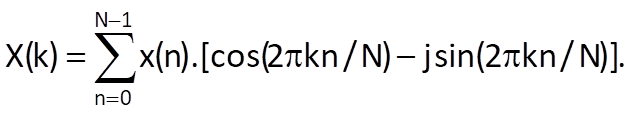
We can use the Euler’s formula to express the definition for the computation of a discrete Fourier transform in the exponential form using the cosine and sine functions:
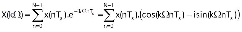
To compute each of the N components of the sequence spectrum, we must perform a N-tuple sum of a product of the time series value with both real and complex components of the transformation kernel, represented by corresponding values of the sine and cosine functions. The computation defined in this way is rather complex and a question arises whether or not it can be optimised.
The computational algorithm can be accelerated by using intermediate results that were computed before or by omitting purposeless calculations, such as the multiplication by zero. Relatively lengthy and repeated computations of values of both trigonometric functions can be facilitated by using precalculated tabular values for one quarter of period in one of both functions. A further increase in efficiency can be achieved by a suitable arrangement of the computational algorithm, for example by the fast Fourier transform.
In order to be able to assess the computational complexity of individual variants of computations of a discrete spectrum from a discrete signal, basic elements of those computations must be determined. As follows from Eq. (4.9), there are two such elements - multiplication of a complex numbers and adding two complex numbers. We will therefore define the unit of computational complexity P by one complex multiplication and by the addition of two complex numbers. Using the above-mentioned definition, the computation of one value of signal spectrum consisting of N samples represents N elements of computational complexity, i.e. N×P. Then the computational complexity for the whole spectrum, consisting of N values, represents the value N×N×P = N2×P. This can be considered as the reference value that can be compared with computational complexities of other variants of computation.
From the computational complexity point of view, the algorithm for fast Fourier transform has two variants that are, in fact, equivalent:
- decomposition in the time domain;
- decomposition in the frequency domain.
First of all, we will look in more detail into the principle of the first variant, which will be then easily applicable to the second variant, too.
Suppose that there is an even number of samples in the input time series. We will divide this sequence into two partial sequences (Figure 4.4):
- {gm} = {x2m} – even elements of the original sequence;
- {hm} = {x2m+1} – odd elements of the original sequence, m = 0,1,…, (N/2)-1.
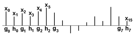
Figure 4.4 Time series decomposition
Furthermore, suppose that all sequences (i.e. original ones and both partial ones) have their own DFTs, which are defined as

and
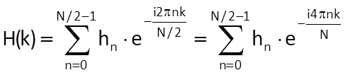
for k ∈ <0, N/2-1>.
Now, let us express the kth value of the spectrum, which was computed by the original transformation algorithm, using intermediate calculations G(k) and H(k). In that case, we can write

If we compute values of the auxiliary partial sequences using the basic definition, the overall computational complexity will be a sum of computational complexities for the computation of spectra of both sequences and their combination:
This means that the computational complexity will be reduced almost to a half if the second term, which expresses the computational complexity of combining both sequences, will be small when compared to the first term (this will be true for large values of N).
And again, if N/2 is even, decomposition can continue. In fact, it is convenient if N is the mth power of two (N = 2m): in that case, decomposition can continue down to the input sequence (Figure 4.5).
Each node in the computational diagram represents a sum of contributions represented by oriented input edges, one of both inputs being multiplied by weight wr. The computational complexity in each node of the diagram will be just P and the number of nodes in each computational layer is N; therefore, the computational complexity in the whole layer is N.P. If N = 2m, the number of layers in the computational diagram will be equal to m = log2N; therefore, the overall computational complexity is N.P.m = N.P.log2N. This expression grows almost linearly for large N, and its values are therefore much smaller than the original computational complexity with a quadratic dependence.
After finishing the decomposition, due to successive decompositions and rearrangements of component input sequences, the samples of input sequence are not arranged in natural order but differently. If we express index values for individual samples in a binary representation and read these binary numbers from right to left, index values will form a naturally increasing sequence. For this reason, the samples of input sequence are arranged in so called binary reversal order.
The existence of standard and repeating butterfly-like computational structures containing four nodes and four edges is another fact facilitating the computation; this means that within each of these component structures, the computation is performed by the same algorithm. Moreover, only input samples of each layer are needed to compute the output values for each layer. Therefore, computations can be performed only for one layer, saving computational memory.

Figure 4.5 Computational diagram of an FFT algorithm by decomposition in the time domain